Chapter 3: Hamiltonian Mechanics

Equations will not display properly in Safari-please use another browser

3.1 From Lagrange to Hamilton

As we saw in Chapter 2, the Lagrangian formulation of the laws of mechanics offers increased flexibility and efficiency relative to the Newtonian methods, and it is based on an appealing principle of least action. In this chapter we add a layer of mathematical sophistication to this formulation of mechanics. The resulting Hamiltonian formulation of the laws of mechanics gives this area of theoretical physics an aura of perfection that has probably not been surpassed by any other area of theoretical physics.

The main goal of the Hamiltonian formulation is to displace the emphasis from the generalized velocities $\dot{q}_a$ to the generalized momenta $p_a$, and from the Lagrangian $L(q_a,\dot{q}_a,t)$ to a new function $H(q_a,p_a,t)$ called the Hamiltonian function of the mechanical system, which is numerically equal to the system's total mechanical energy. The motivation behind this shift of emphasis is clear: While the generalized velocities are rarely conserved quantities, the generalized momenta sometimes are, and while the Lagrangian is never conserved, the Hamiltonian usually is. The Hamiltonian formulation therefore involves all the dynamical quantities that have a chance of being constants of the motion, and this constitutes a useful and interesting refinement of the original Lagrangian methods.

3.1.1 Hamilton's Canonical Equations

To see how the reformulation is accomplished, let us go back to Eq.(2.5.4), which gives the definition of the function $h(q_a,\dot{q}_a,t)$, which is also numerically equal to the total mechanical energy of the system. This is

\begin{equation} h(q_a,\dot{q}_a,t) = \sum_a p_a \dot{q}_a - L(q_a,\dot{q}_a,t), \tag{3.1.1} \end{equation}

where

\begin{equation} p_a = \frac{\partial L}{\partial \dot{q}_a} \tag{3.1.2} \end{equation}

is the generalized momentum associated with the generalized coordinate $q_a$. Notice that here we allow $L$ and $h$ to depend explicitly on time. And notice that the energy function is denoted $h$, not $H$; we will explain this distinction later.

We construct the total differential of $h$:

\[ dh = \sum_a (\dot{q}_a\, d p_a + p_a\, d\dot{q}_a) - dL. \]

To calculate $dL$ we invoke the chain rule, and write

\[ dL = \sum_a \biggl( \frac{\partial L}{\partial q_a} dq_a + \frac{\partial L}{\partial \dot{q}_a} d\dot{q}_a \biggr) + \frac{\partial L}{\partial t} dt. \]

Combining these results gives

\[ dh = \sum_a \biggl[ \dot{q}_a\, dp_a + \biggl( p_a - \frac{\partial L}{\partial \dot{q}_a} \biggr) d\dot{q}_a - \frac{\partial L}{\partial q_a} dq_a \biggr] - \frac{\partial L}{\partial t} dt. \]

From the definition of the generalized momentum we recognize that the coefficient of $d\dot{q}_a$ is zero. And since the Euler-Lagrange (EL) equations can be expressed in the form $\dot{p}_a = \partial L/\partial q_a$, what we have is

\begin{equation} dh = \sum_a ( \dot{q}_a\, dp_a - \dot{p}_a\, dq_a ) - \frac{\partial L}{\partial t} dt. \tag{3.1.3} \end{equation}

Suppose now that $h$ is given as a function of $q_a$, $p_a$, and $t$. Then it would follow as a matter of mathematical identity that the total differential of $h(q_a,p_a,t)$ is

\[ dh = \sum_a \biggl( \frac{\partial h}{\partial q_a} dq_a + \frac{\partial h}{\partial p_a} dp_a \biggr) + \frac{\partial h}{\partial t} dt. \]

Comparing this with Eq.(3.1.3) reveals that we can make the identifications

\[ \dot{q}_a = \frac{\partial h}{\partial p_a}, \qquad \dot{p}_a = -\frac{\partial h}{\partial q_a}, \qquad \frac{\partial L}{\partial t} = -\frac{\partial h}{\partial t}. \]

The first two equations are evolution equations for the dynamical variables $q_a(t)$ and $p_a(t)$. These are almost Hamilton's equations, except for one important subtlety.

The previous identifications can be made if and only if the function $h$ is expressed in terms of $q_a$, $p_a$, and $t$. If it is so expressed, then we have learned that $\dot{q}_a$ is the partial derivative of $h$ with respect to $p_a$ keeping $q_a$ constant, while $\dot{p}_a$ is (minus) the partial derivative of $h$ with respect to $q_a$ keeping $p_a$ constant. Our function $h$, however, has not yet been expressed in terms of the new variables; it is still expressed in terms of the old variables $q_a$, $\dot{q}_a$, and $t$. Before we can write down Hamilton's equations we must solve for $\dot{q}_a$ in terms of $q_a$ and $p_a$, and we must make the substitution in $h$. We must therefore evaluate

\begin{equation} h\bigl(q_a, \dot{q}_a(q_a,p_a), t) \equiv H(q_a,p_a,t), \tag{3.1.4} \end{equation}

and this is what we shall call the Hamiltonian function of the mechanical system. The functions $h$ and $H$ are numerically equal, they both represent the total mechanical energy of the system, but only the Hamiltonian $H$ is the required function of $q_a$, $p_a$, and $t$.

Having clarified this point and made the change of variables from $(q_a,\dot{q}_a)$ to $(q_a,p_a)$, we can finally write down Hamilton's equations,

\begin{equation} \dot{q}_a = \frac{\partial H}{\partial p_a}, \qquad \dot{p}_a = -\frac{\partial H}{\partial q_a}. \tag{3.1.5} \end{equation}

This system of equations is formally equivalent to the original set of EL equations. But instead of representing a set of $n$ second-order differential equations for the coordinates $q_a(t)$ --- there is one equation for each of the $n$ degrees of freedom --- Hamilton's equations represent a set of $2n$ first-order differential equations for the new dynamical variables $q_a(t)$ and $p_a(t)$. The generalized momenta are now put on an equal footing with the generalized coordinates.

The recipe to arrive at Hamilton's canonical equations goes as follows:

Begin with the Lagrangian $L(q_a,\dot{q}_a,t)$ of the mechanical system, expressed in terms of any set of generalized coordinates $q_a$ and the corresponding generalized velocities $\dot{q}_a$. \item Construct the generalized momenta $p_a = \partial L/\partial \dot{q}_a$, and solve for the generalized velocities to obtain $\dot{q}_a(q_a,p_a,t)$.
Construct the Hamiltonian function \[ H(q_a,p_a,t) = \sum_a p_a \dot{q}_a - L \] and express the result entirely in terms of $q_a$, $p_a$, and $t$; at this stage the generalized velocities have completely disappeared from sight.
Formulate Hamilton's equations, \[ \dot{q}_a = \frac{\partial H}{\partial p_a}, \qquad \dot{p}_a = -\frac{\partial H}{\partial q_a} \] and solve the equations of motion for $q_a(t)$ and $p_a(t)$; observe that the generalized velocities $\dot{q}_a$ have reappeared, but now as a consequence of the dynamical equations.

Concrete applications of this recipe will be given in the next section. For the time being we prefer to explore some of the formal consequences of Hamilton's formulation of the laws of mechanics.

3.1.2 Conservation Statements

We begin with an examination of what Hamilton's equations have to say regarding the existence of constants of the motion.

It follows immediately from the dynamical equation

\[ \dot{p}_a = -\frac{\partial H}{\partial q_a} \]

that if the Hamiltonian $H$ happens not to depend explicitly on one of the generalized coordinates, say $q_*$, then $\partial H/\partial q_* = 0$ and $\dot{p}_* = 0$. This means that $p_*$ will be a constant of the motion, and we have established the theorem:

Whenever the Hamiltonian of a mechanical system does not depend explicitly on a generalized coordinate $q_*$, the corresponding generalized momentum $p_*$ is a constant of the motion.

We made a similar statement back in Sec.2.5.1, but in terms of the Lagrangian instead of the Hamiltonian.

Hamilton's equations allow us also to state another theorem, which is very similar: Whenever the Hamiltonian of a mechanical system does not depend explicitly on a generalized momentum $p_*$, the corresponding generalized coordinate $q_*$ is a constant of the motion. This statement is a true consequence of Hamiltonian dynamics, but it is less useful in practice: If $q_*$ were a constant of the motion it is likely that it would not have been selected as a coordinate in the first place!

What do Hamilton's equations have to say about conservation of energy? To answer this let us consider a general Hamiltonian of the form $H(q_a,p_a,t)$, which includes an explicit dependence on $t$. Its total time derivative is

\[ \frac{dH}{dt} = \sum_a \biggl( \frac{\partial H}{\partial q_a} \dot{q}_a + \frac{\partial H}{\partial p_a} \dot{p}_a \biggr) + \frac{\partial H}{\partial t}. \]

By Hamilton's equations this becomes

\[ \frac{dH}{dt} = \sum_a \bigl( -\dot{p}_a \dot{q}_a + \dot{q}_a \dot{p}_a \bigr) + \frac{\partial H}{\partial t}, \]

\begin{equation} \frac{dH}{dt} = \frac{\partial H}{\partial t}. \tag{3.1.6} \end{equation}

Whenever the Hamiltonian of a mechanical system does not depend explicitly on $t$, it is a constant of the motion: $dH/dt = 0$.

Recall that back in Sec.2.5.2 we derived the relation $dh/dt = -\partial L/\partial t$. Here we have instead $dH/dt = \partial H/\partial t$. These statements are compatible by virtue of the fact that $\partial L/\partial t = -\partial H/\partial t$; you will recall that we came across this identification back in Sec.3.1.1.

3.1.3 Phase Space

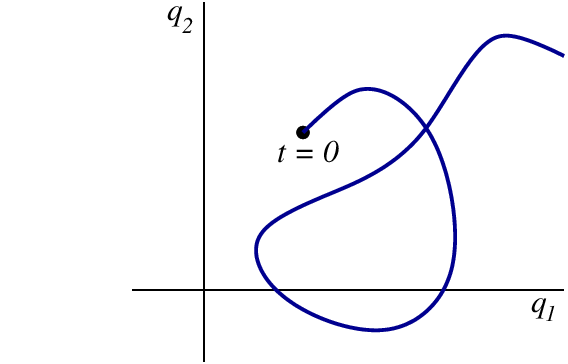
Suppose that a mechanical system possesses $n$ degrees of freedom represented by $n$ generalized coordinates $q_a$ (with $a = 1, 2, \cdots, n$ labeling each one of the $n$ coordinates, as usual). The $n$-dimensional space spanned by the $q_a$'s is called the configuration space of the mechanical system. The motion of the entire system can be represented by a trajectory in configuration space, and the generalized velocities $\dot{q}_a$ represent the tangent to this trajectory. This is illustrated in Fig.3.1. The figure shows that a trajectory in configuration space can cross itself: The system could return later to a position $q_a$ with a different velocity $\dot{q}_a$.

Trajectory in a two-dimensional configuration space — **Figure 3.1:** *A trajectory in a two-dimensional configuration space. It is possible for the trajectory to intersect itself, because the system can go back to the same position after a given interval of time.*

The Hamiltonian formulation of the laws of mechanics gives us an alternative way of representing the motion. Because the coordinates $q_a$ and the momenta $p_a$ are placed on an equal footing, it is natural to form a $2n$-dimensional space that will be spanned by the $n$ coordinates and the $n$ momenta. This new space is called the phase space of the mechanical system. While the phase space is twice as large as the configuration space, it allows a much simpler representation of the motion. The reason is that a point $(q_a,p_a)$ in phase space represents the complete state of motion of a mechanical system at a given time; by identifying the point we obtain the complete information about the positions and momenta of all the particles within the system. (By contrast, in configuration space the complete state of motion would be represented by a point and the tangent to a trajectory that passes through this point.) As the coordinates and momenta change with time the mechanical system traces a trajectory in phase space; each point on this curve represents a new time and a new state of motion. The tangent to a phase-space trajectory gives the phase-space velocity field, $(\dot{q}_a,\dot{p}_a)$. This is illustrated in Fig.3.2.

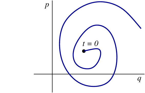
**Figure 3.2:** *A trajectory in a two-dimensional phase space. So long as the Hamiltonian does not depend explicitly on time, it is impossible for the trajectory to intersect itself.*

So long as the Hamiltonian does not depend explicitly on time, a trajectory in phase space can never intersect itself; as we have seen, this is quite unlike a trajectory in configuration space. This property of phase-space trajectories is another reason why motion in phase space is simpler than motion in configuration space. It follows from the fact that the Hamiltonian $H(q_a,p_a)$ is a single-valued function of its arguments: there is only one value of $H$ at each point in phase space. To see the connection, observe that if $H$ is single-valued, then its partial derivatives $\partial H/\partial q_a$ and $\partial H/\partial p_a$ will be single-valued also; and by Hamilton's equations this implies that the tangent $(\dot{q}_a,\dot{p}_a)$ to a phase-space trajectory is a single-valued vector field over phase space. If the tangent of a trajectory is unique at every phase-space point, the trajectory can never intersect itself.

Exercise 3.1: Explain why this conclusion does not apply when the Hamiltonian depends explicitly on time.

When the total energy of the mechanical system is conserved we find that the coordinates and momenta are constrained by the energy equation $H(q_a,p_a) = E = \text{constant}$. In this case the motion will proceed on a fixed ``surface'' in phase space; this ``surface'', which is called an energy surface, has an intrinsic dimensionality of $2n - 1$. The existence of other constants of the motion would also restrict the motion to a ``surface'' of lower dimensionality. We will encounter specific examples of such ``surfaces'' in the next section.

3.1.4 Hamilton's Equations from Hamilton's Principle

Hamilton's equations can be derived directly from Hamilton's principle of least action, $\delta S = 0$. For this purpose the action functional must be expressed in terms of the Hamiltonian instead of the Lagrangian. Because $H = \sum_a p_a \dot{q}_a - L$, we write it as

\[ S = \int_{t_0}^{t_1} L\, dt = \int_{t_0}^{t_1} \biggl( \sum_a p_a \dot{q}_a - H \biggr)\, dt, \]

\begin{equation} S = \int_{t_0}^{t_1} \biggl( \sum_a p_a\, dq_a - H\, dt \biggr). \tag{3.1.7} \end{equation}

The action $S[q_a,p_a]$ must now be thought of as a functional of the variables $q_a(t)$ and $p_a(t)$; all these variables are considered to be independent of each other --- they become connected only after the action has been extremized and the dynamical equations have been imposed. What we have, therefore, is a multi-path functional that depends on $n$ paths $q_a(t)$ and $n$ additional paths $p_a(t)$. Alternatively, we may think of $S[q_a,p_a]$ as a functional of a single path in a $2n$-dimensional phase space.

We intend to compute how the action of Eq.(3.17) changes when the paths are displaced relative to some reference paths $\bar{q}_a(t)$ and $\bar{p}_a(t)$. We will derive the equations of motion by demanding that $\delta S = 0$ to first order in the displacements $\delta q_a(t)$ and $\delta p_a(t)$. We will impose the boundary conditions $\delta q_a(t_0) = \delta q_a(t_1) = 0$: As in the usual form of the variational principle, all paths must begin and end at the same end points in configuration space, $q_a(t_0)$ and $q_a(t_1)$. We will not, however, impose any conditions on the variations $\delta p_a(t)$; these remain completely free, including at $t = t_0$ and $t = t_1$.

The variation of the action is given by

\begin{align} \delta S &= \int_{t_0}^{t_1} \biggl[ \sum_a \bigl( dq_a\, \delta p_a + p_a\, d\delta q_a \bigr) - \sum_a \biggl( \frac{\partial H}{\partial q_a} \delta q_a + \frac{\partial H}{\partial p_a} \delta p_a \biggr)\, dt \biggr] \\ &= \int_{t_0}^{t_1} \sum_a \biggl[ p_a\, d\delta q_a + \biggl( dq_a - \frac{\partial H}{\partial p_a} dt \biggr) \delta p_a - \frac{\partial H}{\partial q_a} dt\, \delta q_a \biggr]. \end{align}

To simplify this we write

\[ p_a\, d \delta q_a = d \bigl( p_a \delta q_a \bigr) - \delta q_a\, d p_a, \]

and we integrate the first term. This gives

\[ \delta S = \sum_a p_a \delta q_a \biggr|^{t_1}_{t_0} + \int_{t_0}^{t_1} \sum_a \biggl[ \biggl( dq_a - \frac{\partial H}{\partial p_a} dt \biggr) \delta p_a - \biggl( dp_a + \frac{\partial H}{\partial q_a} dt \biggr) \delta q_a \biggr], \]

\[ \delta S = \int_{t_0}^{t_1} \sum_a \biggl[ \biggl( \frac{dq_a}{dt} - \frac{\partial H}{\partial p_a} \biggr) \delta p_a - \biggl( \frac{dp_a}{dt} + \frac{\partial H}{\partial q_a} \biggr) \delta q_a \biggr] dt \]

by virtue of the boundary conditions on $\delta q_a(t)$. Because the variations $\delta q_a$ and $\delta p_a$ are arbitrary and independent of each other in the interval $t_0 < t < t_1$, we conclude that

\begin{equation} \delta S = 0 \qquad \Rightarrow \qquad \dot{q}_a = \frac{\partial H}{\partial p_a}, \qquad \dot{p}_a = -\frac{\partial H}{\partial q_a}. \tag{3.1.8} \end{equation}

These are, once more, Hamilton's canonical equations.

3.2 Applications of Hamiltonian Mechanics

3.2.1 Canonical Equations in Cartesian Coordinates

The Lagrangian of a particle moving in a potential $V(x,y,z)$ expressed in Cartesian coordinates is

\begin{equation} L = \frac{1}{2} m ( \dot{x}^2 + \dot{y}^2 + \dot{x}^2 ) - V(x,y,z). \tag{3.2.1} \end{equation}

The momenta are

\[ p_x = \frac{\partial L}{\partial \dot{x}} = m \dot{x} \]

and so on, and the Hamiltonian is $H = p_x \dot{x} + p_y \dot{y} + p_z \dot{z} - L$. Expressing this entirely in terms of the coordinates and momenta, we obtain

\begin{equation} H = \frac{1}{2m} ( p_x^2 + p_y^2 + p_z^2 ) + V(x,y,z). \tag{3.2.2} \end{equation}

At this state the velocities $\dot{x}$, $\dot{y}$, and $\dot{z}$ are no longer part of our description.

The canonical equations are

\[ \dot{x} = \frac{\partial H}{\partial p_x} = \frac{p_x}{m} \]

and so on, as well as

\[ \dot{p}_x = -\frac{\partial H}{\partial x} = -\frac{\partial V}{\partial x} \]

and so on. Summarizing these equations in vectorial form, we have

\begin{equation} \boldsymbol{\dot{r}} = \frac{\boldsymbol{p}}{m}, \qquad \boldsymbol{\dot{p}} = -\boldsymbol{\nabla} V. \tag{3.2.3} \end{equation}

Notice that the first equation reproduces the relationship between $\boldsymbol{p}$ and $\boldsymbol{\dot{r}}$ that was worked out previously. This first-order system of differential equations is of course equivalent to the second-order system $m \boldsymbol{\ddot{r}} = -\boldsymbol{\nabla} V$, which is just Newton's old law; this is obtained by eliminating $\boldsymbol{p}$ from Eqs.(3.2.3).

3.2.2 Canonical Equations in Cylindrical Coordinates

The Lagrangian of a particle moving in a potential $V(\rho,\phi,z)$ expressed in cylindrical coordinates was worked out in Sec.2.4.1. According to Eq.(2.4.3), it is

\begin{equation} L = \frac{1}{2} m ( \dot{\rho}^2 + \rho^2 \dot{\phi}^2 + \dot{z}^2 ) - V(\rho,\phi,z). \tag{3.2.4} \end{equation}

Recall that the cylindrical coordinates are related to the Cartesian coordinates by $x = \rho\cos\phi$, $y = \rho\sin\phi$, and $z=z$.

The momenta are

\begin{align} p_\rho &= \frac{\partial L}{\partial \dot{\rho}} = m \dot{\rho}, \\ p_\phi &= \frac{\partial L}{\partial \dot{\phi}} = m\rho^2 \dot{\phi}, \\ p_z &= \frac{\partial L}{\partial \dot{z}} = m \dot{z}. \end{align}

The Hamiltonian is $H = p_\rho \dot{\rho} + p_\phi \dot{\phi} + p_z \dot{z} - L$. Expressing this entirely in terms of the coordinates and the momenta, we obtain

\begin{equation} H = \frac{1}{2m} \biggl( p_\rho^2 + \frac{p_\phi^2}{\rho^2} + p_z^2 \biggr) + V(\rho,\phi,z). \tag{3.2.5} \end{equation}

At this stage the velocities $\dot{\rho}$, $\dot{\phi}$, and $\dot{z}$ are no longer part of our description.

Exercise 3.2: Go through the algebra that leads to Eq.(3.2.5).

The first set of canonical equations are

\begin{align} \dot{\rho} &= \frac{\partial H}{\partial p_\rho} = \frac{p_\rho}{m}, \tag{3.2.6} \\ \dot{\phi} &= \frac{\partial H}{\partial p_\phi} = \frac{p_\phi}{m\rho^2}, \tag{3.2.7} \\ \dot{z} &= \frac{\partial H}{\partial p_z} = \frac{p_z}{m}. \tag{3.2.8} \end{align}

Notice that these equations reproduce the relationships between the momenta and velocities that were worked out previously. The second set of canonical equations are

\begin{align} \dot{p}_\rho &= -\frac{\partial H}{\partial \rho} = -\frac{\partial V}{\partial \rho} + \frac{p_\phi^2}{m\rho^3}, \tag{3.2.9} \\ \dot{p}_\phi &= -\frac{\partial H}{\partial \phi} = -\frac{\partial V}{\partial \phi}, \tag{3.2.10} \\ \dot{p}_z &= -\frac{\partial H}{\partial z} = -\frac{\partial V}{\partial z}. \tag{3.2.11} \end{align}

If we eliminated the momenta from this system of first-order differential equations we would find that they are equivalent to the second-order equations listed in Eqs.(2.4.4)--(2.4.6).

Exercise 3.3: Verify this last statement.

3.2.3 Canonical Equations in Spherical Coordinates

The Lagrangian of a particle moving in a potential $V(r,\theta,\phi)$ expressed in spherical coordinates was worked out in Sec.2.4.2. According to Eq.(2.4.9), it is

\begin{equation} L = \frac{1}{2} m ( \dot{r}^2 + r^2 \dot{\theta}^2 + r^2\sin^2\theta\, \dot{\phi}^2 ) - V(r,\theta,\phi). \tag{3.2.12} \end{equation}

Recall that the spherical coordinates are related to the Cartesian coordinates by $x = r\sin\theta\cos\phi$, $y = r\sin\theta\sin\phi$, and $z=r\cos\theta$.

The momenta are

\begin{align} p_r &= \frac{\partial L}{\partial \dot{r}} = m \dot{r}, \\ p_\theta &= \frac{\partial L}{\partial \dot{\theta}} = mr^2 \dot{\theta}, \\ p_\phi &= \frac{\partial L}{\partial \dot{\phi}} = m r^2\sin^2\theta\, \dot{\phi}. \end{align}

The Hamiltonian is $H = p_r \dot{r} + p_\theta \dot{\theta} + p_\phi \dot{\phi} - L$. Expressing this entirely in terms of the coordinates and the momenta, we obtain

\begin{equation} H = \frac{1}{2m} \biggl( p_r^2 + \frac{p_\theta^2}{r^2} + \frac{p_\phi^2}{r^2\sin^2\theta} \biggr) + V(r,\theta,\phi). \tag{3.2.13} \end{equation}

At this stage the velocities $\dot{r}$, $\dot{\theta}$, and $\dot{\phi}$ are no longer part of our description.

Exercise 3.4: Go through the algebra that leads to Eq.(3.2.13).

The first set of canonical equations are

\begin{align} \dot{r} &= \frac{\partial H}{\partial p_r} = \frac{p_r}{m}, \label{3.2.14} \\ \dot{\theta} &= \frac{\partial H}{\partial p_\theta} = \frac{p_\theta}{mr^2}, \tag{3.2.15} \\ \dot{\phi} &= \frac{\partial H}{\partial p_\phi} = \frac{p_\phi}{mr^2\sin^2\theta}. \tag{3.2.16} \end{align}

Notice that these equations reproduce the relationships between the momenta and velocities that were worked out previously. The second set of canonical equations are

\begin{align} \dot{p}_r &= -\frac{\partial H}{\partial r} = -\frac{\partial V}{\partial r} + \frac{p_\theta^2}{mr^3} + \frac{p_\phi^2}{mr^3\sin^2\theta}, \tag{3.2.17} \\ \dot{p}_\theta &= -\frac{\partial H}{\partial \theta} = -\frac{\partial V}{\partial \theta} + \frac{p_\phi^2\cos\theta}{mr^2\sin^3\theta}, \tag{3.2.18} \\ \dot{p}_\phi &= -\frac{\partial H}{\partial \phi} = -\frac{\partial V}{\partial \phi}. \tag{3.2.19} \end{align}

If we eliminated the momenta from this system of first-order differential equations we would find that they are equivalent to the second-order equations listed in Eqs.(2.4.10)--(2.4.12).

Exercise 3.5: Verify this last statement.

3.2.4 Planar Pendulum

For our first real application of the Hamiltonian framework we reintroduce the planar pendulum of Sec.1.3.7. The Lagrangian of this mechanical system was first written down in Sec.2.1; it is

\begin{equation} L = m\ell^2 \biggl( \frac{1}{2} \dot{\theta}^2 + \omega^2 \cos\theta \biggr). \tag{3.2.20} \end{equation}

Here $m$ is the mass of the pendulum, $\ell$ is the length of its rigid rod, $\theta$ is the swing angle, and $\omega^2 = g/\ell$, where $g$ is the acceleration of gravity. This mechanical system has a single degree of freedom that is represented by the generalized coordinate $\theta$.

The generalized momentum associated with $\theta$ is

\[ p_\theta = \frac{\partial L}{\partial \dot{\theta}} = m\ell^2 \dot{\theta}, \]

and this equation can be inverted to give $\dot{\theta}$ is terms of $p_\theta$. The pendulum's Hamiltonian is $H = p_\theta \dot{\theta} - L$, or

\begin{equation} H = \frac{p_\theta^2}{2 m\ell^2} - m\ell^2 \omega^2 \cos\theta. \tag{3.2.21} \end{equation}

As usual, we find that at this stage the generalized velocity $\dot{\theta}$ is no longer part of our description.

Exercise 3.6: Verify Eq.(3.2.21).

The canonical equations for the Hamiltonian of Eq.(3.2.21) are

\begin{align} \dot{\theta} &= \frac{\partial H}{\partial p_\theta} = \frac{p_\theta}{m\ell^2}, \tag{3.2.22} \\ \dot{p}_\theta &= -\frac{\partial H}{\partial \theta} = -m\ell^2\omega^2 \sin\theta. \tag{3.2.23} \end{align}

If we eliminate $p_\theta$ from this system of equations we eventually obtain the second-order equation $\ddot{\theta} + \omega^2 \sin\theta = 0$, which is the same as Eq.(1.3.25).

The canonical equations must be integrated numerically if we wish to determine the functions $\theta(t)$ and $p_\theta(t)$. Because they are already presented as a system of first-order differential equations for the set $(\theta,p_\theta)$ of dynamical variables, the numerical techniques introduced in Sec.1.6 can be applied directly. This is one advantage of the Hamiltonian formulation of the laws of mechanics: the first-order form of the equations of motion means that they are directly amenable to numerical integration.

Because the pendulum's Hamiltonian does not depend explicitly on time, it is a constant of the motion. The dynamical variables of the mechanical system are therefore constrained by the equation

\begin{equation} \frac{p_\theta^2}{2m\ell^2} - m\ell^2\omega^2\cos\theta = E = \text{constant}, \tag{3.2.24} \end{equation}

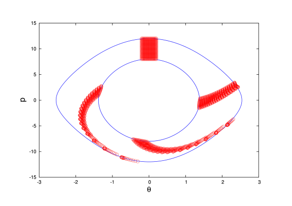
where $E$ is the pendulum's total mechanical energy. This equation describes a one-dimensional curve in the two-dimensional phase space of the mechanical system. This curve is the trajectory of the pendulum in phase space. A number of such phase trajectories are shown in Fig.3.3.

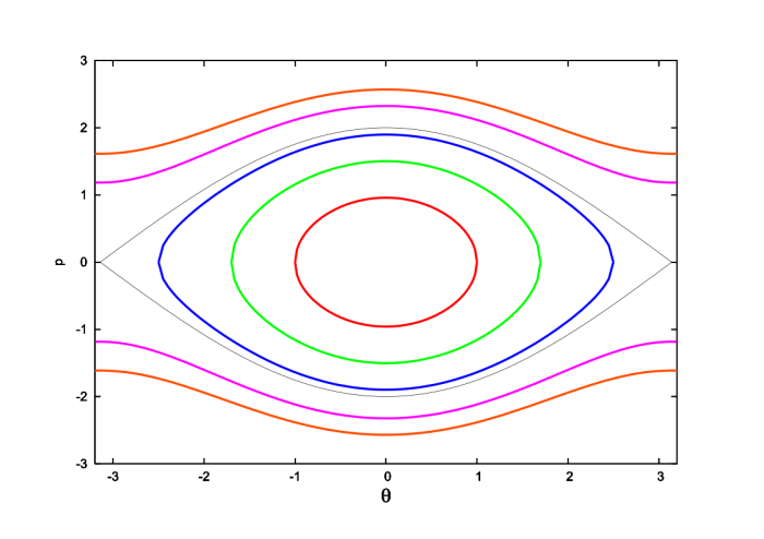
Phase trajectories for a planar pendulum — **Figure 3.3:** Phase trajectories of a planar pendulum. The innermost curves have a rescaled energy $\varepsilon$ smaller than $\omega^2$; they represent the bounded oscillations of a pendulum between the angles $\pm\theta_0$, where $\varepsilon = -\omega^2\cos\theta_0$. The outermost curves have a rescaled energy larger than $\omega^2$; they represent a pendulum undergoing complete revolutions instead of bounded oscillations. The thin black curve represents the marginal case $\varepsilon = \omega^2$.

To describe what is going on in Fig.3.3 it is helpful to introduce the rescaled momentum ${\sf p} = p_\theta/(m\ell^2)$ and the rescaled energy $\varepsilon = E/(m\ell^2)$. In terms of these variables Eq.(3.2.24) becomes

\[ \frac{1}{2} {\sf p}^2 - \omega^2 \cos\theta = \varepsilon, \]

and the phase trajectories are obtained by solving this for ${\sf p}(\theta)$. There are two solutions, one for which ${\sf p}$ is positive, and the other for which ${\sf p}$ is negative.

When $\varepsilon < \omega^2$ we find that the momentum vanishes whenever $\theta = \pm \theta_0$; the amplitude $\theta_0$ of the motion is determined by $\varepsilon = -\omega^2\cos\theta_0$. The motion is then limited to the interval $-\theta_0 \leq \theta \leq \theta_0$, and we have the usual situation of a pendulum oscillating back and forth between the limits $\pm\theta_0$. The phase trajectories representing this bounded, oscillatory motion are closed curves that pass through ${\sf p} = 0$ whenever $\theta$ achieves its limiting values $\pm\theta_0$. The fact that these phase trajectories are closed reflects the fact that the motion of the pendulum is periodic.

When $\varepsilon > \omega^2$ we find that turning points can no longer occur: ${\sf p}$ never changes sign, and $\theta(t)$ increases (or decreases) monotonically. In this case the pendulum does not oscillate; instead it undergoes complete revolutions. The phase trajectories representing this unbounded motion are open curves in the two-dimensional phase space.

The phase trajectory that represents the motion of a pendulum with $\varepsilon = \omega^2$ separates the closed curves that represent oscillatory motion and the open curves that represent the complete revolutions. This curve is called a separatrix.

3.2.5 Spherical Pendulum

We next turn to the spherical pendulum, a mechanical system with two degrees of freedom. Its Lagrangian was derived in Sec.2.2.4; according to Eq.(2.4.19), it is

\[ L = m\ell^2 \biggl( \frac{1}{2} \dot{\theta}^2 + \frac{1}{2} \sin^2\theta\, \dot{\phi}^2 + \omega^2\cos\theta \biggr). \]

Here $m$ is the mass of the pendulum, $\ell$ is the length of its rigid rod, $\theta$ and $\phi$ give the angular position of the pendulum (the angles are defined in Fig.2.10), and $\omega^2 = g/\ell$. The factor $m\ell^2$ in $L$ multiplies each term, and its purpose is simply to give an overall scale to the Lagrangian; the factor accomplishes nothing else, and it would just come along for the ride in our further developments. To save ourselves some trouble we will eliminate this factor by rescaling our quantities. Thus we will deal with the rescaled Lagrangian ${\sf L} = L/(m\ell^2)$, the rescaled momenta ${\sf p}_\theta = p_\theta/(m\ell^2)$ and ${\sf p}_\phi = p_\phi/(m\ell^2)$, and the rescaled Hamiltonian ${\sf H} = H/(m\ell^2)$.

The (rescaled) Lagrangian is

\begin{equation} {\sf L} = \frac{1}{2} \dot{\theta}^2 + \frac{1}{2} \sin^2\theta\, \dot{\phi}^2 + \omega^2\cos\theta, \tag{3.2.25} \end{equation}

and the (rescaled) momenta are

\begin{align} {\sf p}_\theta &= \frac{\partial {\sf L}}{\partial \dot{\theta}} = \dot{\theta} \\ {\sf p}_\phi &= \frac{\partial {\sf L}}{\partial \dot{\phi}} = \sin^2\theta\, \dot{\phi}. \end{align}

The (rescaled) Hamiltonian is ${\sf H} = {\sf p}_\theta \dot{\theta} + {\sf p}_\phi \dot{\phi} - {\sf L}$, and this becomes

\begin{equation} {\sf H} = \frac{1}{2} {\sf p}_\theta^2 + \frac{{\sf p}_\phi^2}{2\sin^2\theta} - \omega^2 \cos\theta \tag{3.2.26} \end{equation}

after expressing the velocities in terms of the momenta.

Exercise 3.7: Verify Eq.(3.2.26).

The canonical equations are

\begin{align} \dot{\theta} &= \frac{\partial {\sf H}}{\partial {\sf p}_\theta} = {\sf p}_\theta, \tag{3.2.27} \\ \dot{\phi} &= \frac{\partial {\sf H}}{\partial {\sf p}_\phi} = \frac{{\sf p}_\phi}{\sin^2\theta}, \tag{3.2.28} \\ \dot{\sf p}_\theta &= -\frac{\partial {\sf H}}{\partial \theta} = \frac{{\sf p}_\phi^2 \cos\theta}{\sin^3\theta} - \omega^2\sin\theta, \tag{3.2.29} \\ \dot{\sf p}_\phi &= -\frac{\partial {\sf H}}{\partial \phi} = 0. \tag{3.2.30} \end{align}

The last equation implies that ${\sf p}_\phi$ is a constant of the motion; we shall set ${\sf p}_\phi = h = \text{constant}$, as we have done in Eq.(2.4.21). Equations (3.2.27) and (3.2.29) must be integrated numerically to determine the functions $\theta(t)$ and ${\sf p}_\theta(t)$; when these are known Eq.(3.2.28) can be integrated for $\phi(t)$.

Exercise 3.8: Show that Eqs.(3.2.27) and (3.2.29) are equivalent to the second-order differential equation of Eq.(2.4.20).

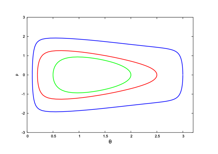
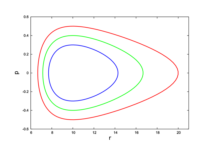
The motion of the spherical pendulum in phase space can be described analytically. Because ${\sf p}_\phi \equiv h$ and ${\sf H} \equiv \varepsilon$ are constants of the motion, the phase trajectories are described by

\begin{equation} \frac{1}{2} {\sf p}_\theta^2 + \frac{h^2}{2\sin^2\theta} - \omega^2 \cos\theta = \varepsilon. \tag{3.2.31} \end{equation}

This equation can be solved for ${\sf p}_\theta$, and the resulting curves are displayed in Fig.3.4. Here the motion always takes place within the bounded interval $\theta_- < \theta < \theta_+$, where the limits $\theta_\pm$ are determined by the values of $h$ and $\varepsilon$ (the details are provided in Sec.2.4.4). It should be noted that the phase space of the spherical pendulum is, strictly speaking, four-dimensional, because it is spanned by the coordinates $\theta$, $p_\theta$, $\phi$, and $p_\phi$. We have reduced this to an effective two-dimensional phase space by examining a ``surface'' $p_\phi = \text{constant} = h$, and by discarding the $\phi$ direction.

Phase trajectories for a spherical pendulum — **Figure 3.4:** Phase trajectories of a spherical pendulum. The different curves have different values of $\varepsilon$ but they share the same value of $h$. The fact that all the trajectories are closed indicates that the motion is always bounded and periodic.

3.2.6 Rotating Pendulum

The rotating pendulum was first examined in Sec.2.4.5. Here we have a planar pendulum whose pivot point is attached to a centrifuge: it rotates with an angular velocity $\Omega$ on a circle of radius $a$. The Lagrangian of this mechanical system is displayed in Eq.(2.4.25):

\[ L = \frac{1}{2} m \Bigl[ (a\Omega)^2 + 2 a \ell \Omega \dot{\theta} \sin(\theta - \Omega t) + \ell^2 \dot{\theta}^2 \Bigr] - m \ell \omega^2 (a \sin\Omega t - \ell \cos\theta). \]

Before we proceed we simplify this Lagrangian using the rules derived in Sec.2.5.3: We discard the term $\frac{1}{2} m (a\Omega)^2$ because it is merely a constant, and we discard the term $-m\ell\omega^2 a \sin\Omega t$ because it is the time derivative of $(m\ell\omega^2a/\Omega) \cos\Omega t$. The simplified Lagrangian is

\[ L = m\ell^2 \biggl[ \frac{1}{2} \dot{\theta}^2 + \frac{a\Omega\dot{\theta}}{\ell} \sin(\theta - \Omega t) + \omega^2 \cos\theta \biggr]. \]

We simplify this further by rescaling away the common factor of $m\ell^2$. Our final (rescaled) Lagrangian is therefore

\begin{equation} {\sf L} = \frac{1}{2} \dot{\theta}^2 + \frac{a\Omega\dot{\theta}}{\ell} \sin(\theta - \Omega t) + \omega^2 \cos\theta. \tag{3.2.32} \end{equation}

It is noteworthy that this Lagrangian depends explicitly on time; this comes as consequence of the fact that the pendulum is driven at a frequency $\Omega$.

The (rescaled) momentum associated with $\theta$ is

\[ {\sf p} = \frac{\partial {\sf L}}{\partial \dot{\theta}} = \dot{\theta} + \frac{a\Omega}{\ell} \sin(\theta - \Omega t). \]

Notice that this is not simply equal to $\dot{\theta}$; here the momentum differs in an essential way from the generalized velocity. The (rescaled) Hamiltonian is ${\sf H} = {\sf p} \dot{\theta} - {\sf L}$. After expressing $\dot{\theta}$ in terms of ${\sf p}$, this becomes

\begin{equation} {\sf H} = \frac{1}{2} \biggl[ {\sf p} - \frac{a\Omega}{\ell} \sin(\theta-\Omega t) \biggr]^2 - \omega^2\cos\theta. \tag{3.2.33} \end{equation}

Exercise 3.9: Verify Eq.(3.2.33).

The canonical equations are

\begin{align} \dot{\theta} &= \frac{\partial {\sf H}}{\partial {\sf p}} = {\sf p} - \frac{a\Omega}{\ell}\sin(\theta - \Omega t), \tag{3.2.34} \\ \dot{\sf p} &= -\frac{\partial {\sf H}}{\partial \theta} = \frac{a\Omega}{\ell} \cos(\theta-\Omega t) \biggl[ {\sf p} - \frac{a\Omega}{\ell}\sin(\theta - \Omega t) \biggr] - \omega^2\sin\theta. \tag{3.2.35} \end{align}

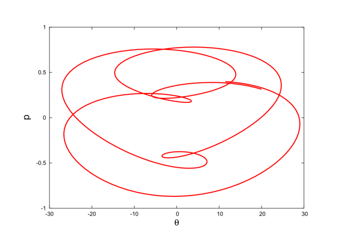
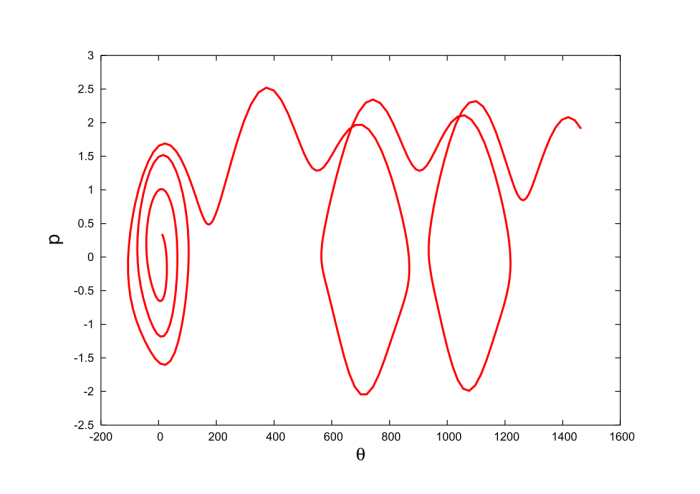
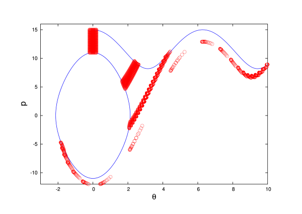
These equations must be integrated numerically, and the results can be displayed as curves in the two-dimensional phase space spanned by the generalized coordinate $\theta$ and its (rescaled) momentum ${\sf p}$. This is done in Fig.3.5 for selected values of $\Omega/\omega$.

Exercise 3.10: Show that Eqs.(3.2.34) and (3.2.35) are equivalent to Eq.(2.4.26).

Phase space trajectory for a rotating pendulum driven by a frequency 0.4 omega — **Figure 3.5:** Phase trajectories of a rotating pendulum. The upper graph shows the motion in phase space of a pendulum driven at a frequency $\Omega = 0.4\omega$; the motion in configuration space can be seen in the upper graph of Fig.2.14. The lower graph has $\Omega = 0.9\omega$ instead, and the motion in configuration space can be seen in Fig.2.15. In both cases we set $(a/\ell)\Omega^2 = 0.2$ and use the same initial conditions as in Figs.2.14 and 2.15. The motion in the upper graph is always confined to the interval $-30^\circ < \theta < 30^\circ$. The motion in the lower graph is not bounded: After oscillating a few times the pendulum is driven to go through a number of complete revolutions before going back to a brief oscillation cycle. In both cases the phase trajectories intersect themselves; this is possible because the Hamiltonian depends explicitly on time.

Phase space trajectory for a rotating pendulum driven at frequency 0.9 omega — **Figure 3.5:** Phase trajectories of a rotating pendulum. The upper graph shows the motion in phase space of a pendulum driven at a frequency $\Omega = 0.4\omega$; the motion in configuration space can be seen in the upper graph of Fig.2.14. The lower graph has $\Omega = 0.9\omega$ instead, and the motion in configuration space can be seen in Fig.2.15. In both cases we set $(a/\ell)\Omega^2 = 0.2$ and use the same initial conditions as in Figs.2.14 and 2.15. The motion in the upper graph is always confined to the interval $-30^\circ < \theta < 30^\circ$. The motion in the lower graph is not bounded: After oscillating a few times the pendulum is driven to go through a number of complete revolutions before going back to a brief oscillation cycle. In both cases the phase trajectories intersect themselves; this is possible because the Hamiltonian depends explicitly on time.

3.2.7 Rolling Disk

The rolling disk was first examined in Sec.2.4.6. Its Lagrangian was obtained in Eq.(2.4.30) and it is

\[ L = \frac{3}{4} m R^2 \dot{\theta}^2 - mg(\ell - R\theta)\sin\alpha. \]

Here $m$ is the mass of the disk, $R$ its radius, $\ell$ is the total length of the inclined plane, and $\alpha$ is the inclination angle; the disk's motion is represented by the angle $\theta$, and these quantities are all illustrated in Fig.2.16. We can simplify the Lagrangian by discarding the constant term $-mg\ell\sin\alpha$; we obtain

\begin{equation} L = \frac{3}{4} m R^2 \dot{\theta}^2 + mgR\sin\alpha\, \theta. \tag{3.2.36} \end{equation}

The momentum associated with $\theta$ is $p \equiv p_\theta = \partial L/\partial \dot{\theta} = \frac{3}{2} m R^2 \dot{\theta}$, and the Hamiltonian is $H = p\dot{\theta} - L$, or

\begin{equation} H = \frac{p^2}{3mR^2} - m g R\sin\alpha\, \theta \tag{3.2.37} \end{equation}

after expressing $\dot{\theta}$ in terms of $p$.

Exercise 3.11: Verify Eq.(3.2.37).

The canonical equations are

\begin{align} \dot{\theta} &= \frac{\partial H}{\partial p} = \frac{2p}{3mR^2}, \tag{3.2.38} \\ \dot{p} &= -\frac{\partial H}{\partial \theta} = mgR\sin\alpha. \tag{3.2.39} \end{align}

By eliminating $p$ from this system of equations we obtain $\ddot{\theta} = \frac{2}{3} g\sin\alpha/R$, which is the same as Eq.(2.4.31). A particular solution to this second-order differential equation was displayed in Eq.(2.4.32). From this solution it is easy to calculate $p(t)$.

Phase trajectories for a rolling disk — **Figure 3.6:** *Phase trajectories of a rolling disk. The curves with $p$ positive represent a disk rolling down the inclined plane. The curves with $p$ negative represent a disk rolling up.*

Exercise 3.12: Obtain the solution to the canonical equations which enforces the initial conditions $\theta(t=0) = 0$ and $p(t=0) = p_0$, where $p_0$ is an arbitrary constant. Plot the motion of the disk in phase space for selected values of $p_0$, and verify that your plots look similar to those featured in Fig.3.6. Finally, show that the phase trajectories are described by the equation

\[ p^2 - 3m^2 g R^3\sin\alpha\, \theta = 3 m R^2 E, \]

where $E$ is the disk's total mechanical energy; find the relationship between $E$ and $p_0$.

3.2.8 Kepler's Problem

revisited in Sec.2.4.7, where the Lagrangian of two bodies subjected to their mutual gravity was decomposed into a centre-of-mass Lagrangian that governs the overall motion of the centre of mass, and a relative Lagrangian that governs the relative separation $\boldsymbol{r}$ between the two bodies. The relative Lagrangian was expressed in polar coordinates in Eq.(2.4.36), which we copy here:

\begin{equation} L = \frac{1}{2} \mu (\dot{r}^2 + r^2 \dot{\phi}^2) + \frac{G\mu M}{r}. \tag{3.2.40} \end{equation}

The quantity $\mu = m_1 m_2 /(m_1 + m_2)$ is the reduced mass of the gravitating system, and $M = m_1 + m_2$ is the total mass. The distance between the two bodies is $r$, and $\phi$ is the orbital angle. Our effective one-body system possesses two degrees of freedom.

The momenta associated with $r$ and $\phi$ are

\begin{align} p_r &= \frac{\partial L}{\partial \dot{r}} = \mu \dot{r}, \\ p_\phi &= \frac{\partial L}{\partial \dot{\phi}} = \mu r^2 \dot{\phi}, \end{align}

and the Hamiltonian is $H = p_r \dot{r} + p_\phi \dot{\phi} - L$, or

\begin{equation} H = \frac{p_r^2}{2\mu} + \frac{p_\phi^2}{2\mu r^2} - \frac{G\mu M}{r} \tag{3.2.41} \end{equation}

after eliminating the velocities in favour of the momenta.

Exercise 3.13: Verify Eq.(3.2.41).

The canonical equations are

\begin{align} \dot{r} &= \frac{\partial H}{\partial p_r} = \frac{p_r}{\mu}, \tag{3.2.42} \\ \dot{\phi} &= \frac{\partial H}{\partial p_\phi} = \frac{p_\phi}{\mu r^2}, \tag{3.2.43} \\ \dot{p}_r &= -\frac{\partial H}{\partial r} = \frac{p_\phi^2}{\mu r^3} - \frac{G\mu M}{r^2}, \tag{3.2.44} \\ \dot{p}_\phi &= -\frac{\partial H}{\partial \phi} = 0. \tag{3.2.45} \end{align}

The last equation implies that $p_\phi$ is a constant of the motion; we shall express this as $p_\phi/\mu = h = \text{constant}$, as we have done in Eq.(2.4.38). Equations (3.2.42) and (3.2.44) can be shown to be equivalent to Eq.(2.4.37).

Exercise 3.14: Verify this last statement.

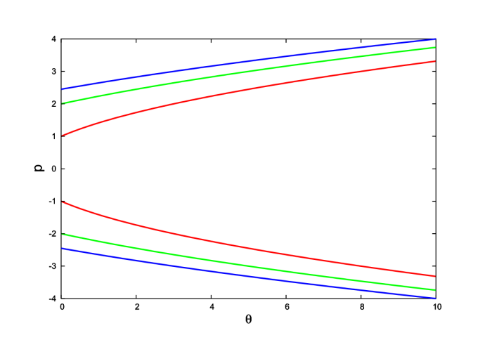
The solutions to the equations of motion were studied back in Sec.1.5. The motion in phase space is described by the equation $H = E = \text{constant}$, which expresses the fact that $H$ also is a constant of the motion. Introducing the rescaled quantities ${\sf p} = p_r/\mu$ and $\varepsilon = E/\mu$, this equation states that

\[ \frac{1}{2} {\sf p}^2 + \frac{h^2}{2r^2} - \frac{GM}{r} = \varepsilon. \]

This equation can be solved for ${\sf p}$ and the result is displayed in Fig.3.7.

Phase trajectories for Kepler's problem — **Figure 3.7:** Phase trajectories of Kepler's problem, in a two-dimensional subspace of the complete four-dimensional phase space. The different curves have different values of $\varepsilon$ but they share the same value of $h$. The fact that all the trajectories are closed indicates that the motion is bounded and periodic. The curves are most easily produced by using the results of Sec.~\ref{i.5.9}: We use the parametric representation $r = p/(1 + e\cos\phi)$ and ${\sf p} = \dot{r} = e \sqrt{GM/p} \sin\phi$, where $p$ is the semilatus rectum and $e$ the eccentricity. In terms of these we have $h = \sqrt{GMp}$ and $\varepsilon = -GM(1-e^2)/(2p)$. The phase trajectories displayed here have eccentricities of 0.3, 0.4, and 0.5, respectively; they all share the same value of $p$.

3.2.9 Charged Particle in an Electromagnetic Field

For our last application we consider a particle of charge $q$ moving in an electric field $\boldsymbol{E}$ and a magnetic field $\boldsymbol{B}$. The fields can be expressed as $\boldsymbol{E} = -\partial \boldsymbol{A}/\partial t - \boldsymbol{\nabla} \Phi$ and $\boldsymbol{B} = \boldsymbol{\nabla} \times \boldsymbol{A}$ in terms of potentials $\Phi$ and $\boldsymbol{A}$; and as we saw in Sec.2.6, the Lagrangian of the particle is

\begin{equation} L = \frac{1}{2} m v^2 - q \Phi + q \boldsymbol{A} \cdot \boldsymbol{v}, \tag{3.2.46} \end{equation}

where $v^2 = \boldsymbol{v} \cdot \boldsymbol{v} = \dot{x}^2 + \dot{y}^2 + \dot{z}^2$. The momentum vector $\boldsymbol{p}$ associated with the position vector $\boldsymbol{r}$ was obtained back in Eq.(2.6.5); it is $\boldsymbol{p} = m \boldsymbol{v} + q \boldsymbol{A}$. The Hamiltonian is $H = \boldsymbol{p} \cdot \boldsymbol{v} - L$, or

\begin{equation} H = \frac{1}{2m} (\boldsymbol{p} - q\boldsymbol{A}) \cdot (\boldsymbol{p} - q \boldsymbol{A}) + q\Phi. \tag{3.2.47} \end{equation}

Exercise 3.15: Verify Eq.(3.2.47).

The canonical equations governing the evolution of $x$ and $p_x$ are

\begin{align} \dot{x} &= \frac{\partial H}{\partial p_x} = \frac{1}{m} (p_x - q A_x), \tag{3.2.48} \\ \dot{p}_x &= -\frac{\partial H}{\partial x} = \frac{q}{m} (\boldsymbol{p} - q\boldsymbol{A}) \cdot \frac{\partial \boldsymbol{A}}{\partial x} - q \frac{\partial \Phi}{\partial x}, \tag{3.2.49} \end{align}

and similar equations can be obtained for the pairs $(y,p_y)$ and $(z,p_z)$. The second-order differential equation that is obtained by eliminating $p_x$ from the system of Eqs.(3.2.48) and (3.2.49) is

\[ m \ddot{x} = q (\boldsymbol{E} + \boldsymbol{v} \times \boldsymbol{B})_x, \]

and this is the $x$ component of the Lorentz-force law. The other components are obtained by similar manipulations.

Exercise 3.16: Go through the algebra that leads to Eqs.(3.2.48) and (3.2.49), and then repeat these calculations for the other four canonical equations. Finally, show that these equations are indeed equivalent to the Lorentz-force law, $m\boldsymbol{\ddot{x}} = q(\boldsymbol{E} + \boldsymbol{v} \times \boldsymbol{B})$. Be warned: this last calculation can be a bit tricky!

3.3 Liouville's Theorem

3.3.1 Formulation of the Theorem

We wish to examine the motion of a large number $N$ of identical particles in phase space; each particle has its own position and momentum, but all are subjected to the same potential $V$. We may imagine that the $N$ particles co-exist peacefully, without interacting with one another. Or we may imagine that the $N$ particles are in fact mental copies of one and the same particle, on which we are carrying out $N$ separate experiments. In all cases we shall refer to the $N$ particles as an ensemble of particles, and we wish to follow the motion of this ensemble in phase space.

Supposing (for concreteness) that each particle possesses three degrees of freedom, which it would if it were to move in a three-dimensional space, we could form a $6N$-dimensional phase space of all positions and momenta of all the particles, and we could display the motion of the whole ensemble as a trajectory in this super phase space. We shall not follow this strategy, although it is a viable one. Instead, we will simultaneously represent the motion of all $N$ particles in the six-dimensional phase space of an individual particle (which one we pick does not matter, because the particles are all identical); this individual phase space is spanned by the three position variables and the three momentum variables. We will have, therefore, a collection of $N$ separate trajectories in phase space.

We have seen that a point in phase space --- the phase space of an individual particle --- gives a complete representation of the state of motion of that particle at an instant of time. By identifying the point we automatically know the particle's position and momentum, and this is all there is to know about the state of motion of the particle at that instant of time; the equations of motion then tell us how the state of motion will change from this time to the next time. As was mentioned previously, the particle will trace a trajectory in phase space, and each point on this curve will represent a state of motion corresponding to a given instant of time.

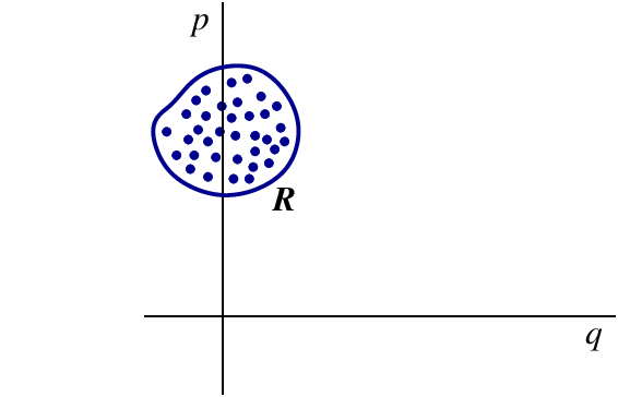
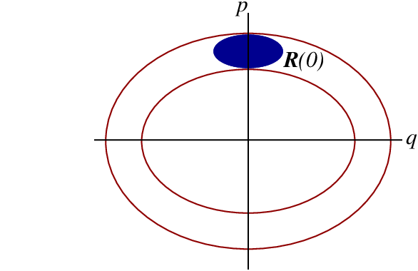
Suppose that we wish to represent, at an initial moment $t=0$, the state of motion of our ensemble of $N$ particles, and that we wish to do so in the phase space of an individual particle. We will need to identify $N$ points in the phase space, and each of these points will represent the state of motion of one of the particles. We will call them representative points. Because we give each particle its own set of initial conditions, the representative points will be spread out in phase space, and they will define a region ${\cal R}$ of phase space. We will assume that this region is bounded; this is illustrated in Fig.3.8.

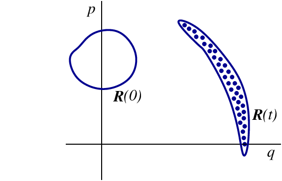
**Figure 3.8:** The initial state of motion of an ensemble of $N$ identical particles is represented by $N$ representative points in the phase space of an individual particle. These points are distributed within a bounded region ${\cal R}$ of the phase space.

Each particle within the ensemble moves according to Hamilton's equations, and each representative point traces a trajectory in phase space. Because the initial conditions are different for each particle, each trajectory is different. In a time $t$ the initial region ${\cal R}(0)$ of phase space will be mapped to a distinct region ${\cal R}(t)$; this mapping is illustrated in Fig.3.9. The shape of ${\cal R}(t)$ will in general be very different from the shape of the initial region ${\cal R}(0)$. But according to Liouville's theorem:

The ``volume'' of the region ${\cal R}(t)$ of phase space,

\[ V = \int_{{\cal R}(t)} dq_1 dq_2 \cdots dp_1 dp_2 \cdots, \]

is independent of the time $t$; the volume does not change as the region ${\cal R}(t)$ evolves in accordance with the motion of each representative point in phase space.

So Liouville's theorem states that while the Hamiltonian evolution of the ensemble will produce a deformation of the region ${\cal R}(t)$, the evolution will nevertheless preserve its ``volume'', as defined by the integration over ${\cal R}(t)$ of the ``volume element'' $dV = dq_1 dq_2 \cdots dp_1 dp_2 \cdots$ in phase space.

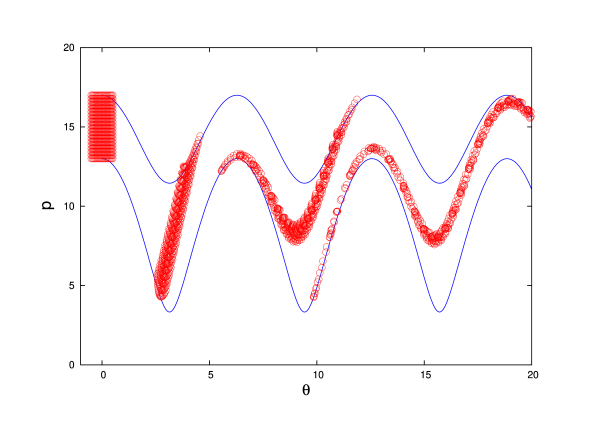
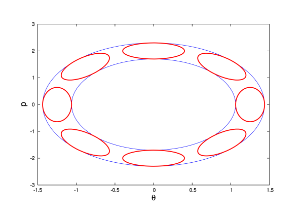
**Figure 3.9:** An initial region ${\cal R}(0)$ of phase space containing the $N$ representative points is mapped by Hamilton's equations to a new region ${\cal R}(t)$. The shape of the new region can be very different from the shape of the initial region. But according to Liouville's theorem, their phase-space ``volumes'' are equal.

The proof of this important theorem will be presented below. Illustrations of the theorem are displayed in Fig.3.10, which shows how an initial region ${\cal R}(0)$ of a two-dimensional phase space evolves over time. It is important to note that Liouville's theorem is formulated in phase space, and that its validity is therefore restricted to phase space. An attempt to formulate such a theorem in configuration space, or in a position-velocity space, would fail: Volumes in such spaces are not preserved under the time evolution of the ensemble.

**Figure 3.10:** Evolution of a region ${\cal R}(t)$ in a two-dimensional phase space; the mechanical system is the planar pendulum of Sec.3.2.4. For all three plots the initial region ${\cal R}(0)$ is the rectangular region near the top of the page, and ${\cal R}(t)$ is drawn at three successive times. Each region consists of 400 representative points, drawn as open circles, and the motion of each point in phase space is determined by numerical integration of Hamilton's equations. Two bounding phase trajectories are also shown to guide the eye. In the first (upper) graph the initial conditions are such that the motion each pendulum is bounded, limited to an interval $-\theta_0 < \theta < \theta_0$. In the second (middle) graph the initial conditions are such that the motion of each pendulum is not bounded; each goes through complete revolutions. In the third (lower) graph the initial conditions are such that about half the pendula undergo bounded motion, while the other half undergo unbounded motion. All three graphs reveal a significant distortion of the region ${\cal R}(t)$ as the motion of each pendulum proceeds; but the area of this region is the same at all times.

Evolution of a region in phase space relating to the motion of a planar pendulum. The initial conditions are such that the motion of each pendulum is not bounded — **Figure 3.10:** Evolution of a region ${\cal R}(t)$ in a two-dimensional phase space; the mechanical system is the planar pendulum of Sec.3.2.4. For all three plots the initial region ${\cal R}(0)$ is the rectangular region near the top of the page, and ${\cal R}(t)$ is drawn at three successive times. Each region consists of 400 representative points, drawn as open circles, and the motion of each point in phase space is determined by numerical integration of Hamilton's equations. Two bounding phase trajectories are also shown to guide the eye. In the first (upper) graph the initial conditions are such that the motion each pendulum is bounded, limited to an interval $-\theta_0 < \theta < \theta_0$. In the second (middle) graph the initial conditions are such that the motion of each pendulum is not bounded; each goes through complete revolutions. In the third (lower) graph the initial conditions are such that about half the pendula undergo bounded motion, while the other half undergo unbounded motion. All three graphs reveal a significant distortion of the region ${\cal R}(t)$ as the motion of each pendulum proceeds; but the area of this region is the same at all times.

3.3.2 Case Study: Linear Pendulum

The examples displayed in Fig.3.10 involved a nonlinear pendulum, and the nonlinearities of the dynamics produced interesting distortions of the initial (rectangular) region ${\cal R}(0)$ of the system's phase space. These distortions, however, are difficult (probably impossible) to describe mathematically, and this means that the validity of Liouville's theorem would be difficult to check directly.

To help build confidence in these new ideas we will simplify the problem further and eliminate the nonlinear aspects of the dynamics. We will therefore examine the motion of an ensemble of linear pendula. Each pendulum possesses the Hamiltonian

\begin{equation} H = \frac{1}{2} p^2 + \frac{1}{2} \omega^2 \theta^2, \tag{3.3.1} \end{equation}

which can be obtained from Eq.(3.2.21) by (i) invoking the approximation $\cos\theta = 1 - \frac{1}{2} \theta^2$, (ii) discarding an irrelevant constant term, and (iii) rescaling the variables according to $H/(m\ell^2) \to H$ and $p_\theta/(m\ell^2) \to p_\theta \equiv p$.

The canonical equations are

\begin{equation} \dot{\theta} = p, \qquad \dot{p} = -\omega^2 \theta, \tag{3.3.2} \end{equation}

and they are equivalent to the second-order differential equation $\ddot{\theta} + \omega^2 \theta = 0$ that governs simple harmonic motion. The general solution to Eqs.(3.3.2) is

\begin{align} \theta(t) &= \theta(0) \cos\omega t + \frac{p(0)}{\omega} \sin\omega t, \tag{3.3.3} \\ p(t) &= p(0) \cos\omega t - \omega \theta(0) \sin\omega t, \tag{3.3.4} \end{align}

where $\theta(0) \equiv \theta(t=0)$ is the initial position of a pendulum sampled from the ensemble, and $p(0) \equiv p(t=0)$ is its initial momentum. The energy of each pendulum is conserved, and the trajectory of each pendulum in phase space is an ellipse described by

\[ \frac{1}{2} p^2 + \frac{1}{2} \omega^2 \theta^2 = \varepsilon = \frac{1}{2} p^2(0) + \frac{1}{2} \omega^2 \theta^2(0). \]

By varying the initial conditions among all the pendula within the ensemble, we trace ellipses of varying shapes and sizes.

Each pendulum within the ensemble has its own set of initial conditions $\theta(0)$ and $p(0)$. The spread of initial conditions in phase space defines the initial region ${\cal R}(0)$. Suppose that we choose initial conditions such that the $N$ values for $\theta(0)$ are centered around $\theta(0) = 0$ and are within a deviation $\sigma_\theta$ away from zero, either in the negative or positive direction. Suppose also that the $N$ values for $p(0)$ are centered around $p(0) = p_0$ and are within a deviation $\sigma_p$ away from $p_0$. What we have, then, is a region ${\cal R}(0)$ in phase space that is centered at $(\theta,p) = (0,p_0)$ and has a typical extension of $\sigma_\theta$ in the position direction, and a typical extension of $\sigma_p$ is the momentum direction. This region will evolve to ${\cal R}(t)$ in a time $t$, as each pendulum within the ensemble moves in phase space. We wish to describe this evolution, and in particular, we wish to show that the ``volume'' of ${\cal R}(t)$ is independent of time.

Concretely we choose the boundary of ${\cal R}(0)$ to be described by an ellipse of semiaxes $\sigma_\theta$ and $\sigma_p$, centered at $\theta(0) = 0$ and $p(0) = p_0$. (It is important to understand that this ellipse has nothing to do with the elliptical motion of each pendulum in phase space. We have two unrelated ellipses: one representing the motion of each pendulum in phase space, the other representing the distribution of initial conditions.) We describe this boundary by the parametric equations

\begin{equation} \theta(0;\alpha) = -\sigma_\theta \cos\alpha, \qquad p(0;\alpha) = p_0 + \sigma_p \sin\alpha, \tag{3.3.5} \end{equation}

in which the parameter $\alpha$ ranges from $0$ to $2\pi$. All the representative points are initially located within this ellipse, and the region ${\cal R}(0)$ is therefore a solid ellipse; this is illustrated in Fig.3.11. The phase-space ``volume'' of this region is, in this two-dimensional context, the surface area of the solid ellipse. This ``volume'' can be calculated as

\begin{align} V(0) &= \int_{{\cal R}(0)} d\theta(0) dp(0) \\ &=\int_{-\sigma_\theta}^{\sigma_\theta} p_+(0)\, d\theta(0) + \int_{\sigma_\theta}^{-\sigma_\theta} p_-(0)\, d\theta(0). \end{align}

The first integral is the area under the upper branch of the ellipse (the one for which $p \geq p_0$), and the second integral is (minus) the area under the lower branch (the one for which $p \leq p_0$). This can be expressed cleanly as

\begin{align} V(0) &= \int_0^{2\pi} p(0;\alpha) \frac{d\theta(0;\alpha)}{d\alpha}\, d\alpha \\ &= \int_0^{2\pi} \bigl[ p_0 + \sigma_p \sin\alpha \bigr] \bigl[ \sigma_\theta \sin\alpha \bigr]\, d\alpha, \end{align}

and integration gives

\begin{equation} V(0) = \pi \sigma_\theta \sigma_p, \tag{3.3.6} \end{equation}

the expected result for an ellipse of semiaxes $\sigma_\theta$ and $\sigma_0$. This is the phase-space ``volume'' of our initial region ${\cal R}(0)$. We now wish to determine how this region evolves in time, and how its volume changes.

The phase space volume is defined by the surface area of a solid elipse — **Figure 3.11:** The initial region ${\cal R}(0)$ in phase space has an elliptical boundary. The ellipse is centered at $(\theta,p) = (0,p_0)$ and it has semiaxes $\sigma_\theta$ and $\sigma_p$. An angle $\alpha$ (not shown) parameterizes the position on the boundary.

Exercise 3.17: Verify Eq.(3.3.6).

**Figure 3.12:** The initial region ${\cal R}(0)$ in phase space is mapped to a new region ${\cal R}(t)$ after a time $t$. These regions are shown for $\omega t = 0$ (uppermost ellipse), $\omega t = \pi/4$, $\omega t = \pi/2$ (rightmost ellipse), $\omega t = 3\pi/4$, and so on.

As time moves forward each point $\theta(0;\alpha)$, $p(0;\alpha)$ on the boundary of the region ${\cal R}(0)$ is mapped to a corresponding point $\theta(t;\alpha)$, $p(t;\alpha)$ on the boundary of the new region ${\cal R}(t)$. The coordinates of the new point are given by Eqs.(3.3.3) and (3.3.4), which we write as

\begin{align} \theta(t;\alpha) &= \theta(0;\alpha) \cos\omega t + \frac{p(0;\alpha)}{\omega} \sin\omega t, \tag{3.3.7} \\ p(t;\alpha) &= p(0;\alpha) \cos\omega t - \omega \theta(0;\alpha) \sin\omega t. \tag{3.3.8} \end{align}

The new regions ${\cal R}(t)$ are displayed in Fig.3.12 for selected values of $t$. Their ``volume'' is given by

\begin{align} V(t) &= \int_{{\cal R}(t)} d\theta(t) dp(t) \\ &= \int_0^{2\pi} p(t;\alpha) \frac{d\theta(t;\alpha)}{d\alpha}\, d\alpha. \end{align}

After involving Eqs.(3.3.7), (3.3.8) and performing the integration, we arrive at

\begin{equation} V(t) = \pi \sigma_\theta \sigma_p, \tag{3.3.9} \end{equation}

the same result as in Eq.(3.3.6). The volume of the phase-space region ${\cal R}(t)$ is indeed independent of time.

Exercise 3.18: Go through the calculational steps that lead to Eq.(3.3.9).

3.3.3 Proof of Liouvilles's

There are, in fact, two versions of Liouville's theorem. The first version is concerned with a quantity $\rho$, the density of representative points in phase space, which we shall introduce below; it states that under a Hamiltonian evolution,

\begin{equation} \frac{d\rho}{dt} = 0, \tag{3.3.10} \end{equation}

so that $\rho$ is a constant of the motion. The second version is concerned with the volume $V(t)$ of a region ${\cal R}(t)$ of phase space that is defined by an ensemble of representative points; it states that $V(t)$ is constant under a Hamiltonian evolution. The second version of the theorem is a corollary of the first. We will prove the first version first, and then obtain the second version.

We have a region ${\cal R}(t)$ of phase space that contains a large number $N$ of representative points; this region has a volume $V = \int_{{\cal R}(t)} dV$, where $dV = dq_1 dq_2 \cdots dp_1 dp_2 \cdots$ is the element of phase-space volume. We imagine that $N$ is sufficiently large that we can introduce a notion of phase-space density $\rho$ of representative points; this, by definition, is the number $dN$ of representative points contained within a small region of phase space, divided by its volume $dV$. We have, therefore, $\rho = dN/dV$, and the density can vary from point to point in phase space: $\rho = \rho(q_a,p_a,t)$; we also allow the density to depend explicitly on time.

The phase-space density $\rho$ plays essentially the same role here as the density of electric charge $\rho_e$ plays in electromagnetism. If we introduce a velocity field $\boldsymbol{v} = (\dot{q}_1,\dot{q}_2,\cdots, \dot{p}_1, \dot{p}_2,\cdots)$ in phase space, then the current density $\boldsymbol{j} = \rho \boldsymbol{v}$ will play essentially the same role here as the electric current density $\boldsymbol{j}_e$ plays in electromagnetism. It is known that in electromagnetism, the charge and current densities are related by an equation of continuity,

\[ \frac{\partial \rho_e}{\partial t} + \boldsymbol{\nabla} \cdot \boldsymbol{j}_e = 0. \]

We will show that a very similar equation of continuity applies to $\rho$ and $\boldsymbol{j}$ in phase space. In electromagnetism the equation of continuity is a differential statement of charge conservation; in phase space it will be a differential statement of the fact that the number of representative points is conserved.

Exercise 3.18: Consult your favorite textbook on electromagnetism and review its derivation of the equation of continuity for electric charge.

Consider a region $V$ of phase space which is bounded by the ``surface'' $S$. This region is completely arbitrary, but it is assumed to be fixed in time; unlike the region ${\cal R}(t)$ considered previously, this one does not move around in phase space. The representative points contained in ${\cal R}(t)$ do move, however, and in time they will move in and out of the region $V$. The number of representative points contained in $V$ at any given time $t$ is given by the phase-space integral $\int_V \rho\, dV$. The number of representative points that {\it move out} of $V$ per unit time is then given by

\[ -\frac{d}{dt} \int_V \rho\, dV. \]

If the total number of representative points is to be conserved, this number must be equal to the number of representative points that cross the bounding surface $S$, in the outward direction, per unit time. By definition of the current density $\boldsymbol{j}$, this is

\[ \oint_S \boldsymbol{j} \cdot d\boldsymbol{a}, \]

where $d\boldsymbol{a}$ is an element of ``surface area'' in phase space; this vector is directed along the outward normal to the surface, and its magnitude is equal to the area of an element of surface in phase space. Equating these two expressions gives

\[ -\int_V \frac{\partial \rho}{\partial t}\, dV = \oint_S (\rho \boldsymbol{v}) \cdot d\boldsymbol{a}. \]

We next use the phase-space version of Gauss's theorem to express the right-hand side as a volume integral,

\[ \int_V \boldsymbol{\nabla} \cdot (\rho \boldsymbol{v})\, dV, \]

where $\boldsymbol{\nabla} = (\partial/\partial q_1, \partial/\partial q_2, \cdots, \partial/\partial p_1, \partial/\partial p_2, \cdots)$ is the gradient operator in phase space. We now have

\[ \int_V \biggl[ \frac{\partial \rho}{\partial t} + \boldsymbol{\nabla} \cdot (\rho \boldsymbol{v}) \biggr] dV = 0, \]

since this equation must be valid for all regions $V$ of phase space, we conclude that

\[ \frac{\partial \rho}{\partial t} + \boldsymbol{\nabla} \cdot (\rho \boldsymbol{v}) = 0. \]

This is the phase-space version of the equation of continuity.

A more explicit form of the equation of continuity is

\[ 0 = \frac{\partial \rho}{\partial t} + \frac{\partial}{\partial q_1} \bigl( \rho \dot{q}_1 \bigr) + \frac{\partial}{\partial q_2} \bigl( \rho \dot{q}_2 \bigr) + \cdots + \frac{\partial}{\partial p_1} \bigl( \rho \dot{p}_1 \bigr) + \frac{\partial}{\partial p_2} \bigl( \rho \dot{p}_2 \bigr) + \cdots, \]

\[ 0 = \frac{\partial \rho}{\partial t} + \sum_a \biggl[ \frac{\partial}{\partial q_a} \bigl( \rho \dot{q}_a \bigr) + \frac{\partial}{\partial p_a} \bigl( \rho \dot{p}_a \bigr) \biggr]. \]

The phase-space coordinates of the representative points change in accordance with Hamilton's equations. We may therefore substitute $\dot{q}_a = \partial H/\partial p_a$ and $\dot{p}_a = -\partial H/\partial q_a$ into the preceding equation. We obtain

\begin{align} 0 &= \frac{\partial \rho}{\partial t} + \sum_a \biggl[ \frac{\partial}{\partial q_a} \biggl( \rho \frac{\partial H}{\partial p_a} \biggr) - \frac{\partial}{\partial p_a} \biggl( \rho \frac{\partial H}{\partial q_a} \biggr) \biggr] \\ &= \frac{\partial \rho}{\partial t} + \sum_a \biggl[ \frac{\partial \rho}{\partial q_a} \frac{\partial H}{\partial p_a} - \frac{\partial \rho}{\partial p_a} \frac{\partial H}{\partial q_a} + \rho \biggl( \frac{\partial^2 H}{\partial q_a \partial p_a} - \frac{\partial^2 H}{\partial p_a \partial q_a} \biggr) \biggr] \\ &= \frac{\partial \rho}{\partial t} + \sum_a \biggl[ \frac{\partial \rho}{\partial q_a} \frac{\partial H}{\partial p_a} - \frac{\partial \rho}{\partial p_a} \frac{\partial H}{\partial q_a} \biggr], \end{align}

\[ 0 = \frac{\partial \rho}{\partial t} + \sum_a \biggl[ \frac{\partial \rho}{\partial q_a} \dot{q}_a + \frac{\partial \rho}{\partial p_a} \dot{p}_a \biggr] \]

after involving Hamilton's equations one more time.

have obtained the first version of Liouville's theorem: If the phase-space density $\rho$ is a function of $q_a$, $p_a$, and $t$, then by virtue of the chain rule its total time derivative is

\begin{equation} \frac{d\rho}{dt} = \sum_a \biggl[ \frac{\partial \rho}{\partial q_a} \dot{q}_a + \frac{\partial \rho}{\partial p_a} \dot{p}_a \biggr] + \frac{\partial \rho}{\partial t}, \tag{3.3.11} \end{equation}

and according to our previous results, this is zero. We have therefore established Eq.(3.3.10) on the basis of the equation of continuity in phase space.

To arrive at the second version of Liouville's theorem, consider the $N$ representative points that are contained in the moving region ${\cal R}(t)$ of phase space. By definition of the phase-space density, we have

\[ N = \int_{{\cal R}(t)} \rho\, dV, \]

and we know that this number is preserved as we follow the evolution of ${\cal R}(t)$ over time. We now also know that the density $\rho$ is a constant of the motion. This means that if, for example, the density is initially chosen to be uniform over ${\cal R}(0)$, then it will stay uniform over ${\cal R}(t)$ throughout the Hamiltonian evolution. In this case we may bring $\rho$ outside of the integral, and we obtain the statement that $N/\rho = \int_{{\cal R}(t)} dV \equiv V(t)$ is preserved during the evolution. This is the second version of Liouville's theorem.

3.3.4 Poisson Brackets

The expression of Eq.(3.3.11) for the total time derivative of the phase-space density,

\begin{align} \frac{d\rho}{dt} &= \frac{\partial \rho}{\partial t} + \sum_a \biggl[ \frac{\partial \rho}{\partial q_a} \dot{q}_a + \frac{\partial \rho}{\partial p_a} \dot{p}_a \biggr] \\ &= \frac{\partial \rho}{\partial t} + \sum_a \biggl[ \frac{\partial \rho}{\partial q_a} \frac{\partial H}{\partial p_a} - \frac{\partial \rho}{\partial p_a} \frac{\partial H}{\partial q_a} \biggr], \end{align}

is in fact a mathematical identity that holds for any function $\rho(q_a,p_a,t)$ defined in phase space. Because this expression is so general, it occurs often, and it has proved convenient to introduce a notation to recast it in a more compact form.

Let $f(q_a,p_a,t)$ and $g(q_a,p_a,t)$ be any two functions on phase space. Their Poisson bracket is defined by

\begin{equation} [f,g] = \sum_a \biggl( \frac{\partial f}{\partial q_a} \frac{\partial g}{\partial p_a} - \frac{\partial f}{\partial p_a} \frac{\partial g}{\partial q_a} \biggr). \tag{3.3.12} \end{equation}

The Poisson bracket possesses the following properties: It is antisymmetric,

\begin{equation} [g,f] = -[f,g]; \tag{3.3.13} \end{equation}

it is linear with respect to each of its arguments,

\begin{equation} [f_1+f_2,g] = [f_1,g] + [f_2,g], \qquad [f,g_1+g_2] = [f,g_1] + [f,g_2]; \tag{3.3.14} \end{equation}

it satisfies the product rule of differential calculus,

\begin{equation} [f_1 f_2, g] = f_1 [f_2,g] + [f_1,g] f_2, \qquad [f, g_1 g_2] = g_1 [f,g_2] + [f,g_1] g_2; \tag{3.3.15} \end{equation}

and finally, it satisfies the Jacobi identity,

\begin{equation} \bigl[ f, [g,h] \bigr] + \bigl[ h, [f,g] \bigr] + \bigl[ g, [h,f] \bigr] = 0. \tag{3.3.16} \end{equation}

Exercise 3.19: Show that these are all true properties of the Poisson bracket. Be warned: To establish the Jacobi identity requires a lengthy calculation.

Particular applications of the Poisson bracket are

\begin{equation} [f,q_a] = -\frac{\partial f}{\partial p_a}, \qquad [f,p_a] = \frac{\partial f}{\partial q_a}. \tag{3.3.17} \end{equation}

Special cases of these identities are

\begin{equation} [q_a,q_b] = 0, \qquad [q_a,p_b] = \delta_{ab}, \qquad [p_a,p_b] = 0. \tag{3.3.18} \end{equation}

Exercise 3.20: Verify Eqs.(3.3.17) and (3.3.18).

In terms of the Poisson bracket, the total derivative with respect to time of a function $f(q_a,p_a,t)$ is given by

\begin{equation} \frac{df}{dt} = \frac{\partial f}{\partial t} + [f,H]. \tag{3.3.19} \end{equation}

If we apply this identity to the Hamiltonian $H$ we obtain $dH/dt = \partial H/\partial t + [H,H] = \partial H/\partial t$, by virtue of the antisymmetric property of the Poisson bracket. If the Hamiltonian does not depend explicitly on time, we obtain the statement $dH/dt = 0$ and the conclusion that the Hamiltonian is a constant of the motion. This is a well-known result by now, but notice how quickly the result follows from the Poisson-bracket formalism.

Exercise 3.21: Verify Eq.(3.3.19). Then show that it leads to the expected answers for $dq_a/dt$ and $dp_a/dt$.

3.4 Canonical Transformation

3.4.1 Introduction

A theme that has been central to our development of Lagrangian and Hamiltonian mechanics is the arbitrariness of the generalized coordinates $q_a$ that are adopted to describe the motion of a mechanical system. The Euler-Lagrange equations

\[ \frac{d}{dt} \frac{\partial L}{\partial \dot{q}_a} - \frac{\partial L}{\partial q_a} = 0 \]

and the canonical equations

\[ \dot{q}_a = \frac{\partial H}{\partial p_a}, \qquad \dot{p}_a = -\frac{\partial H}{\partial q_a} \]

are all invariant under a transformation of the generalized coordinates, from the set $q_a$ of old coordinates to any set $Q_a$ of new coordinates; these can by any functions $Q_a(q_1,q_2,\cdots)$ of the old coordinates.

In this section we show that the Hamiltonian formulation of the laws of mechanics admits a much wider class of possible transformations. In this context it is possible to change the phase-space coordinates from an old set $(q_a,p_a)$ to a new set $(Q_a,P_a)$, with

\begin{equation} Q_a = Q_a(q_1,q_2,\cdots,p_1,p_2,\cdots), \qquad P_a = P_a(q_1,q_2,\cdots,p_1,p_2,\cdots). \tag{3.4.1} \end{equation}

Notice that the new generalized coordinates $Q_a$ are now functions of the old coordinates and the old momenta; the new generalized momenta $P_a$ also are functions of all the old phase-space coordinates. Under some conditions, which will be specified below, such a transformation will leave the canonical equations invariant: In the new system of phase-space coordinates there will exist a transformed Hamiltonian $H'(Q_a,P_a,t)$ such that

\begin{equation} \dot{Q}_a = \frac{\partial H'}{\partial P_a}, \qquad \dot{P}_a = -\frac{\partial H'}{\partial Q_a}. \tag{3.4.2} \end{equation}

Under these conditions the transformation is known as a canonical transformation; transformations of the phase-space coordinates that are not canonical have no value, and they will not be considered.

Canonical transformations have the interesting and useful property that they leave the element of phase-space volume invariant. Thus,

\begin{equation} dV = dq_1 dq_2 \cdots dp_1 dp_2 \cdots = dQ_1 dQ_2 \cdots dP_1 dP_2 \cdots. \tag{3.4.3} \end{equation}

In other words, the Jacobian of the transformation is equal to one. This gives us a means of checking whether a specified transformation is canonical or not: If the Jacobian of the transformation is not equal to one, the transformation is not canonical. This property of canonical transformations is rather deep, and it implies that the validity of Liouville's theorem is not restricted to a particular choice of phase-space coordinates; the volume of a region ${\cal R}(t)$ of phase space is invariant under a canonical transformation.

Because a canonical transformation produces new coordinates that are a mixture of old coordinates and old momenta, they can dramatically alter the physical meaning of the phase-space coordinates. Thus, a given $Q_a$ may not necessarily represent a position variable, and a given $P_a$ may not represent a momentum variable. A trivial example is the canonical transformation $Q_a = p_a$, $P_a = -q_a$, which clearly leaves the canonical equations invariant; here the new coordinates are the old momenta, the new momenta are the old coordinates, and the new phase-space coordinates do not retain their traditional physical meaning. Because the new ``coordinates'' $Q_a$ and the new ``momenta'' $P_a$ may not have straightforward physical interpretations after a canonical transformation, it is customary to refer to the new phase-space coordinates simply as conjugate variables.

3.4.2 Case Study: Linear Pendulum

Before we present the general theory of canonical transformations in the next subsection, we shall take the time to get acquainted with some of the fundamental ideas by examining a specific example. We return once more to the linear pendulum of Sec.3.3.2, with its Hamiltonian

\begin{equation} H = \frac{1}{2} p^2 + \frac{1}{2} \omega^2 q^2, \tag{3.4.4} \end{equation}

where we have identified the generalized coordinate $q$ with the swing angle $\theta$. The canonical equations for this mechanical system are

\begin{equation} \dot{q} = \frac{\partial H}{\partial p} = p, \qquad \dot{p} = -\frac{\partial H}{\partial q} = -\omega^2 q. \tag{3.4.5} \end{equation}

We intend to show that a canonical transformation can turn this rather simple mechanical system into a completely trivial one. Solving for the motion of the trivial system will allow us to find the solution to Eqs.(3.4.5) without having to solve these equations directly. This, in a nutshell, is the power and purpose of canonical transformations.

Let us consider the following transformation of the phase-space coordinates:

\begin{equation} Q = \text{arctan}\Bigl( \frac{\omega q}{p} \Bigr), \qquad P = \frac{1}{2\omega} \bigl( p^2 + \omega^2 q^2 \bigr). \tag{3.4.6} \end{equation}

The new ``momentum'' $P$ is proportional to the Hamiltonian; a curve $P = \text{constant}$ is therefore represented as an ellipse in the old phase space. A curve $Q = \text{constant}$, on the other hand, is represented as a straight line that passes through the origin; this line has a slope $p/q = \omega/\tan Q$, and $Q$ is an angle relative to the $p$ axis. The inverse transformation is

\begin{align} q = \sqrt{\frac{2P}{\omega}}\sin Q, \qquad p = \sqrt{2\omega P} \cos Q. \tag{3.4.7} \end{align}

It is easy to check that the transformation has a unit Jacobian. This is given by

\begin{align} J &= \left| \begin{array}{cc} \partial q/ \partial Q & \partial q/ \partial P \\ \partial p/ \partial Q & \partial p/ \partial P \end{array} \right| = \left| \begin{array}{cc} \sqrt{2P/ \omega} \cos Q & \sin Q/ \sqrt{2\omega P} \\ - \sqrt{2\omega P} \sin Q & \sqrt{\omega/2P} \cos Q \end{array} \right| \\ &= \cos^2 Q + \sin^2 Q = 1, \end{align}

and $J$ is indeed equal to one. This gives us a successful partial check on whether the transformation is properly canonical.

Exercise 3.22: Check that Eq.(3.4.6) is the inverse transformation to Eq.(3.4.7). Then check all the partial derivatives that have been involved in the computation of the Jacobian.

The transformation of Eq.(3.4.6) will be canonical if and only if it preserves the form of the canonical equations. We shall now show that this is indeed the case. We will find that the evolution equations for $Q$ and $P$ are given by

\begin{equation} \dot{Q} = \frac{\partial H}{\partial P} = \omega, \qquad \dot{P} = -\frac{\partial H}{\partial Q} = 0, \tag{3.4.8} \end{equation}

with a Hamiltonian now expressed as

\begin{equation} H = \omega P, \tag{3.4.9} \end{equation}

which follows by substituting Eq.(3.4.6) for $P$ into Eq.(3.4.4) for $H$. In this particular instance of a canonical transformation, the new Hamiltonian $H'$ is the same as the old Hamiltonian $H$.

We can verify the results of Eq.(3.4.8) by computing $\dot{Q}$ and $\dot{P}$ directly from their definitions in Eq.(3.4.6). We begin with the relation $\tan Q = \omega q/p$, which we differentiate with respect to $t$. We get

\[ (1 + \tan^2 Q) \dot{Q} = \frac{\omega \dot{q}}{p} - \frac{\omega q \dot{p}}{p^2}, \]

and if we now involve Eq.(3.4.5), this becomes

\[ (1 + \tan^2 Q) \dot{Q} = \omega \biggl( 1 + \frac{\omega^2 q^2}{p^2} \biggr) = \omega (1 + \tan^2 Q). \]

This gives, finally, $\dot{Q} = \omega$, as we had stated in Eq.(3.4.8). The right-hand side of this equation happens to be equal to $\partial H/\partial P$, and we have recovered one of the two canonical equations. The second equation follows much more easily. Because $P = H/\omega$ it is obvious that its equation of motion is $\dot{P} = 0$, as was stated in Eq.(3.4.8). The right-hand side of this equation happens to be equal to $\partial H/\partial Q$, and we have recovered our second canonical equation.

The main purpose of the canonical transformation of Eq.(3.4.6) is to bring the Hamiltonian to the simple form of Eq.(3.4.9). This Hamiltonian is proportional to the new momentum $P$, and it does not depend on the new coordinate $Q$. As a result, the equations of motion are exceptionally simple, and they can be solved easily: The new momentum is a constant of the motion and the new coordinate $Q$ behaves in time according to $Q(t) = \omega t + \delta$, where $\delta$ is a constant of integration. The transformation has therefore turned the original problem into a very simple one. With the solution to the simple problem in hand, we may return to the original problem and express its solution as

\[ q(t) = \sqrt{\frac{2P}{\omega}}\sin(\omega t + \delta), \qquad p(t) = \sqrt{2\omega P} \cos(\omega t + \delta), \]

by substituting our solution for $Q(t)$ into Eqs.(3.4.7). Our linear pendulum evidently undergoes simple harmonic motion. The frequency of the motion is $\omega$, and its amplitude is $\sqrt{2P/\omega}$.

3.4.3 General Theory of Canonical Transformations

When is a transformation of the phase-space coordinates,

\[ Q_a = Q_a(q_b,p_b,t), \qquad P_a = P_a(q_b,p_b,t), \]

a canonical transformation? The fundamental criterion is that the transformation must preserve the form of Hamilton's canonical equations: The transformation must produce a new Hamiltonian $H'$ such that

\[ \dot{Q}_a = \frac{\partial H'}{\partial P_a}, \qquad \dot{P}_a = -\frac{\partial H'}{\partial Q_a}. \]

The question is: Under what conditions does this occur? We will provide a number of answers to this question, ranging from the formal to the practical.

Let us recall from Sec.3.1.4 that Hamilton's equations for the original set $(q_a,p_a)$ of phase-space coordinates can be derived on the basis of Hamilton's principle of least action. The principle can be expressed in the form

\[ \delta \int_{t_0}^{t_1} \biggl( \sum_a p_a\, dq_a - H\, dt \biggr) = 0; \]

the variations $\delta q_a(t)$, $\delta p_a(t)$ are all independent, and they are subjected to the boundary conditions $\delta q_a(t_0) = \delta q_a(t_1) = 0$. If Hamilton's equations are to hold also for the new set $(Q_a,P_a)$ of phase-space coordinates, they must also follow from Hamilton's principle. We must then have, simultaneously,

\[ \delta \int_{t_0}^{t_1} \biggl( \sum_a P_a\, dQ_a - H'\, dt \biggr) = 0; \]

here it is the variations $\delta Q_a(t)$, $\delta P_a(t)$ that are taken to be independent and subjected to the boundary conditions $\delta Q_a(t_0) = \delta Q_a(t_1) = 0$. The two formulations of Hamilton's principle will be compatible with each other if and only if the integrands $\sum_a p_a\, dq_a - H\, dt$ and $\sum_a P_a\, dQ_a - H'\, dt$ differ by the total derivative $dF_1$ of a function $F_1(q_a,Q_a,t)$ of the old and new coordinates. For we would have, in this case, a difference of integrals given by

\[ \int_{t_0}^{t_1} dF_1 = F_1\bigl( q_a(t_1), Q_a(t_1), t_1 \bigr) - F_1\bigl( q_a(t_0), Q_a(t_0), t_0 \bigr), \]

and $\delta \int_{t_0}^{t_1} dF_1 = 0$ would follow immediately by virtue of the boundary conditions on the variations $\delta q_a$ and $\delta Q_a$.

The first answer to our question is therefore this: A transformation of the phase-space coordinates is a canonical transformation when there exists a function $F_1(q_a,Q_a,t)$ such that

\begin{equation} \sum_a p_a\, dq_a - H\, dt = \sum_a P_a\, dQ_a - H'\, dt + dF_1. \tag{3.4.10} \end{equation}

The function $F_1(q_a,Q_a,t)$ is called the generating function of the canonical transformation. This is a formal answer to our question; we will provide more practical answers at a later stage.

The total derivative of $F_1$ can be expressed as

\[ dF_1 = \sum_a \frac{\partial F_1}{\partial q_a} dq_a + \sum_a \frac{\partial F_1}{\partial Q_a} dQ_a + \frac{\partial F_1}{\partial t} dt. \]

On the other hand, Eq.(3.4.10) can be rewritten as

\[ dF_1 = \sum_a p_a\, dq_a - \sum_a P_a\, dQ_a + (H'-H)\, dt. \]

Because both equations must be true, we obtain the identifications

\begin{equation} p_a = \frac{\partial F_1}{\partial q_a}, \qquad P_a = -\frac{\partial F_1}{\partial Q_a}, \qquad H' = H + \frac{\partial F_1}{\partial t}. \tag{3.4.11} \end{equation}

The first two equations give us the old momenta $p_a$ and the new momenta $P_a$ in terms of the derivatives of the generating function. The last equation gives us the new Hamiltonian $H'$; if the generating function does not depend explicitly on time, the new Hamiltonian is the same as the old.

As a trivial application of the foregoing, let us consider the generating function $F_1 = \sum_b q_b Q_b$. The old momenta are $p_a = \partial F_1/\partial q_a = Q_a$ and the new momenta are $P_a = -\partial F_1/\partial Q_a = -q_a$. This generating function therefore produces the trivial transformation $Q_a = p_a$, $P_a = -q_a$ that was encountered previously. This is a canonical transformation because it is generated by the function $F_1$. Because this function does not depend explicitly on time, the transformation does not change the Hamiltonian: $H' = H$. And the transformation, evidently, preserves the form of the canonical equations.

A more interesting application involves the function $F_1 = \frac{1}{2} \omega q^2 \text{cotan} Q$, which generates the transformation of Eqs.(3.4.6) and (3.4.7). We have

\[ p = \frac{\partial F_1}{\partial q} = \omega q\, \text{cotan} Q = \frac{\omega q}{\tan Q} \]

and

\[ P = -\frac{\partial F_1}{\partial Q} = \frac{1}{2} \omega q^2 (1 + \text{cotan}^2 Q) = \frac{1}{2} \omega q^2 \biggl( 1 + \frac{p^2}{\omega^2 q^2} \biggr) = \frac{1}{2\omega} (p^2 + \omega^2 q^2), \]

as was anticipated in Eqs.(3.4.6). Because $F_1$ does not depend explicitly on $t$, we have that $H' = H = \omega P$, as was stated in Eq.(3.4.9).

3.4.4 Alternative Generating Functions

It is possible to introduce new generating functions that depend on an alternative choice of variables. Consider, for example, the new function

\[ F_2 = F_1 + \sum_a Q_a P_a. \]

Its total derivative is

\begin{align} dF_2 &= dF_1 + \sum_a P_a\, dQ_a + \sum_a Q_a\, dP_a \\ &= \sum_a p_a\, dq_a - \sum_a P_a\, dQ_a + (H'-H)\, dt + \sum_a P_a\, dQ_a + \sum_a Q_a\, dP_a \\ &= \sum_a p_a\, dq_a + \sum_a Q_a\, dP_a + (H'-H)\, dt; \end{align}

in the second line we substituted a previous expression for $dF_1$, and in the last line we canceled out the terms $\sum_a P_a\, dQ_a$. The fact that $dF_2$ involves the differentials $dq_a$, $dP_a$, and $dt$ informs us that $F_2$ must be a function of $q_a$, $P_a$, and $t$. We have, therefore,

\begin{equation} F_2 = F_1 + \sum_a Q_a P_a = F_2(q_a,P_a,t), \tag{3.4.12} \end{equation}

and this new generating function does indeed depend on a different set of variables. Our previous calculation allows us to make the identifications

\begin{equation} p_a = \frac{\partial F_2}{\partial q_a}, \qquad Q_a = \frac{\partial F_2}{\partial P_a}, \qquad H' = H + \frac{\partial F_2}{\partial t}. \tag{3.4.13} \end{equation}

This freedom to introduce alternative generating functions adds flexibility to the framework of canonical transformations. We will make use of this in the next section.

Exercise 3.23: Consider the new generating function $F_3 = F_1 - \sum_a q_a p_a$. On which variables does $F_3$ depend? Find expressions for $P_a$, $q_a$, and $H'$ in terms of partial derivatives of $F_3$.

Exercise 3.24: Consider now the new generating function $F_4 = F_1 + \sum_a Q_a P_a - \sum_a q_a p_a$. On which variables does $F_4$ depend? Find expressions for $q_a$, $Q_a$, and $H'$ in terms of partial derivatives of $F_4$.

3.4.5 Direct Conditions

It is rarely convenient to test whether a transformation is canonical by attempting to find its generating function. More direct tests are available, fortunately, and these do not require knowledge of the generating function. We shall describe these tests in this and the following subsection. For simplicity we assume that the transformation does not depend explicitly on time; this means that $H' = H$.

The transformation $Q_a = Q_a(q_b,p_b)$ implies that the time derivative of the new coordinates can be expressed as

\begin{align} \dot{Q}_a &= \sum_b \frac{\partial Q_a}{\partial q_b} \dot{q}_b + \sum_b \frac{\partial Q_a}{\partial p_b} \dot{p}_b \\ &= \sum_b \frac{\partial Q_a}{\partial q_b} \frac{\partial H}{\partial p_b} - \sum_b \frac{\partial Q_a}{\partial p_b} \frac{\partial H}{\partial q_b}. \end{align}

If the transformation is canonical, this will be equal to $\partial H /\partial P_a$. With $H$ written as a function of the old phase-space coordinates, this is

\[ \frac{\partial H}{\partial P_a} = \sum_b \frac{\partial H}{\partial q_b} \frac{\partial q_b}{\partial P_a} + \sum_b \frac{\partial H}{\partial p_b} \frac{\partial p_b}{\partial P_a}. \]

Hamilton's equations therefore imply

\begin{align} 0 &= \dot{Q}_a - \frac{\partial H}{\partial P_a} \\ &= \sum_b \biggl( \frac{\partial Q_a}{\partial q_b} - \frac{\partial p_b}{\partial P_a} \biggr) \frac{\partial H}{\partial p_b} - \sum_b \biggl( \frac{\partial Q_a}{\partial p_b} + \frac{\partial q_b}{\partial P_a} \biggr) \frac{\partial H}{\partial q_b}. \end{align}

This equation will be satisfied if and only if

\begin{equation} \frac{\partial}{\partial q_b} Q_a(q_b,p_b) = \frac{\partial}{\partial P_a} p_b(Q_a,P_a), \qquad \frac{\partial}{\partial p_b} Q_a(q_b,p_b) = -\frac{\partial}{\partial P_a} q_b(Q_a,P_a). \tag{3.4.14} \end{equation}

This first set of conditions must therefore be met if the transformation is to be a canonical transformation.

The second set of conditions is obtained by starting instead with the transformation $P_a = P_a(q_b,p_b)$. This time we have

\begin{align} \dot{P}_a &= \sum_b \frac{\partial P_a}{\partial q_b} \dot{q}_b + \sum_b \frac{\partial P_a}{\partial p_b} \dot{p}_b \\ &= \sum_b \frac{\partial P_a}{\partial q_b} \frac{\partial H}{\partial p_b} - \sum_b \frac{\partial P_a}{\partial p_b} \frac{\partial H}{\partial q_b}. \end{align}

If the transformation is canonical, this will be equal to $-\partial H /\partial Q_a$. With $H$ written as a function of the old phase-space coordinates, this is

\[ \frac{\partial H}{\partial Q_a} = \sum_b \frac{\partial H}{\partial q_b} \frac{\partial q_b}{\partial Q_a} + \sum_b \frac{\partial H}{\partial p_b} \frac{\partial p_b}{\partial Q_a}. \]

Hamilton's equations therefore imply

\begin{align} 0 &= \dot{P}_a + \frac{\partial H}{\partial Q_a} \\ &= \sum_b \biggl( \frac{\partial P_a}{\partial q_b} + \frac{\partial p_b}{\partial Q_a} \biggr) \frac{\partial H}{\partial p_b} - \sum_b \biggl( \frac{\partial P_a}{\partial p_b} - \frac{\partial q_b}{\partial Q_a} \biggr) \frac{\partial H}{\partial q_b}. \end{align}

This equation will be satisfied if and only if

\begin{equation} \frac{\partial}{\partial q_b} P_a(q_b,p_b) = -\frac{\partial}{\partial Q_a} p_b(Q_a,P_a), \qquad \frac{\partial}{\partial p_b} P_a(q_b,p_b) = \frac{\partial}{\partial Q_a} q_b(Q_a,P_a). \tag{3.4.15} \end{equation}

This is the second set of conditions that must be met if the transformation is to be a canonical transformation.

Equations (3.4.15) and (3.4.14) are called the direct conditions for a canonical transformation: all these conditions will be satisfied if the transformation $Q_a(q_a,p_a)$ and $P_a(q_a,p_a)$ is a canonical transformation. For a mechanical system with $n$ degrees of freedom we have a total of $4n^2$ conditions. As we shall see, these are not all independent. In the next subsection we will identify a smaller, and more convenient, set of necessary and sufficient conditions.

3.4.6 Canonical Invariants

As was stated in Sec.3.4.1, a canonical transformation has the property of leaving the element of phase-space volume invariant:

\begin{equation} dV = dq_1 dq_2 \cdots dp_1 dp_2 \cdots = dQ_1 dQ_2 \cdots dP_1 dP_2 \cdots . \tag{3.4.16} \end{equation}

A canonical transformation of the phase-space coordinates therefore has a unit Jacobian, $J = 1$. This statement can be shown to be a consequence of the direct conditions, Eqs.(3.4.14) and (3.4.15).

Another consequence of the direct conditions is the fact that canonical transformations leave all Poisson brackets invariant. Thus, if

\[ [f,g]_{q,p} = \sum_a \biggl( \frac{\partial f}{\partial q_a} \frac{\partial g}{\partial p_a} - \frac{\partial f}{\partial p_a} \frac{\partial g}{\partial q_a} \biggr) \]

is the Poisson bracket in the old phase-space coordinates, and if

\[ [f,g]_{Q,P} = \sum_a \biggl( \frac{\partial f}{\partial Q_a} \frac{\partial g}{\partial P_a} - \frac{\partial f}{\partial P_a} \frac{\partial g}{\partial Q_a} \biggr) \]

is the Poisson bracket in the new coordinates, then

\begin{equation} [f,g]_{q,p} = [f,g]_{Q,P} \tag{3.4.17} \end{equation}

if the transformation is canonical.

It is this statement which provides us with an efficient method to test whether a transformation $Q_a = Q_a(q_b,p_b,t)$, $P_a = P_a(q_b,p_b,t)$ is canonical: By virtue of the automatic relations (refer back to Sec.3.3.4)

\[ [Q_a,Q_b]_{Q,P} = 0, \qquad [Q_a,P_b]_{Q,P} = \delta_{ab}, \qquad [P_a,P_b]_{Q,P} = 0 \]

and the invariance of the Poisson bracket, we must have that the relations

\begin{equation} [Q_a,Q_b]_{q,p} = 0, \qquad [Q_a,P_b]_{q,p} = \delta_{ab}, \qquad [P_a,P_b]_{q,p} = 0 \tag{3.4.18} \end{equation}

hold if the transformation is canonical. Similarly, a transformation $q_a = q_a(Q_b,P_b,t)$, $p_a = p_a(Q_b,P_b,t)$ is canonical if the Poisson-bracket relations

\begin{equation} [q_a,q_b]_{Q,P} = 0, \qquad [q_a,p_b]_{Q,P} = \delta_{ab}, \qquad [p_a,p_b]_{Q,P} = 0 \tag{3.4.19} \end{equation}

are satisfied. The conditions of Eqs.(3.4.18) or (3.4.19) can be shown to be sufficient and necessary. For a mechanical system with $n$ degrees of freedom, we have a total of $(2n-1)n$ conditions to satisfy; when $n = 1$ there is only one relevant condition, $[Q,P]_{q,p} = 1$ or $[q,p]_{Q,P} = 1$.

Exercise 3.25: Verify that $[Q,P]_{q,p} = 1$ in the case of the canonical transformation presented in Sec.3.4.2.

We will not present a general proof of the statements that the phase-space volume element and the Poisson bracket are canonical invariants. We will, instead, present a proof that is restricted to a two-dimensional phase space. The restricted proof is easy to produce; the general proof would be much more difficult.

We consider a canonical transformation of the form $Q = Q(q,p)$, $P = P(q,p)$. The direct conditions for this transformation are

\[ \frac{\partial Q}{\partial q} = \frac{\partial p}{\partial P}, \qquad \frac{\partial Q}{\partial p} = -\frac{\partial q}{\partial P}, \qquad \frac{\partial P}{\partial q} = -\frac{\partial p}{\partial Q}, \qquad \frac{\partial P}{\partial p} = \frac{\partial q}{\partial Q}. \]

The volume elements are related by

\[ dq dp = |J|\, dQ dP, \qquad dQ dP = |J|^{-1}\, dqdp, \]

in which $J$ is the Jacobian of the transformation, and $J^{-1}$ its inverse. The Jacobian is

\[ J = \left| \begin{array}{cc} \partial q/\partial Q & \partial q/\partial P \\ \partial p/\partial Q & \partial p/\partial P \end{array} \right | = \frac{\partial q}{\partial Q} \frac{\partial p}{\partial P} - \frac{\partial q}{\partial P} \frac{\partial p}{\partial Q}. \]

Its inverse is

\[ J^{-1} = \left| \begin{array}{cc} \partial Q/\partial q & \partial Q/\partial p \\ \partial P/\partial q & \partial P/\partial p \end{array} \right | = \frac{\partial Q}{\partial q} \frac{\partial P}{\partial p} - \frac{\partial Q}{\partial p} \frac{\partial P}{\partial q}. \]

By involving the direct conditions we may write this as

\[ J^{-1} = \frac{\partial p}{\partial P} \frac{\partial q}{\partial Q} - \frac{\partial q}{\partial P} \frac{\partial p}{\partial Q}, \]

and this is equal to $J$. We therefore have $J^{-1} = J$, or $J^2 = 1$, and we conclude that $|J| = 1$. This proves that the volume element is indeed preserved under a canonical transformation.

The Poisson bracket in the new phase-space coordinates is

\[ [f,g]_{Q,P} = \frac{\partial f}{\partial Q} \frac{\partial g}{\partial P} - \frac{\partial f}{\partial P} \frac{\partial g}{\partial Q}. \]

If we consider $f$ and $g$ to be functions of $q$ and $p$, we may use the chain rule and express this as

\begin{align} [f,g]_{Q,P} &= \biggl( \frac{\partial f}{\partial q} \frac{\partial q}{\partial Q} + \frac{\partial f}{\partial p} \frac{\partial p}{\partial Q} \biggr) \biggl( \frac{\partial g}{\partial q} \frac{\partial q}{\partial P} + \frac{\partial g}{\partial p} \frac{\partial p}{\partial P} \biggr) - \biggl( \frac{\partial f}{\partial q} \frac{\partial q}{\partial P} + \frac{\partial f}{\partial p} \frac{\partial p}{\partial P} \biggr) \biggl( \frac{\partial g}{\partial q} \frac{\partial q}{\partial Q} + \frac{\partial g}{\partial p} \frac{\partial p}{\partial Q} \biggr) \\ &= \frac{\partial f}{\partial q} \frac{\partial g}{\partial q} \biggl( \frac{\partial q}{\partial Q} \frac{\partial q}{\partial P} - \frac{\partial q}{\partial P} \frac{\partial q}{\partial Q} \biggr) + \frac{\partial f}{\partial q} \frac{\partial g}{\partial p} \biggl( \frac{\partial q}{\partial Q} \frac{\partial p}{\partial P} - \frac{\partial q}{\partial P} \frac{\partial p}{\partial Q} \biggr) + \frac{\partial f}{\partial p} \frac{\partial g}{\partial q} \biggl( \frac{\partial p}{\partial Q} \frac{\partial q}{\partial P} - \frac{\partial p}{\partial P} \frac{\partial q}{\partial Q} \biggr) + \frac{\partial f}{\partial p} \frac{\partial g}{\partial p} \biggl( \frac{\partial p}{\partial Q} \frac{\partial p}{\partial P} - \frac{\partial p}{\partial P} \frac{\partial p}{\partial Q} \biggr) \\ &= \biggl( \frac{\partial f}{\partial q} \frac{\partial g}{\partial p} - \frac{\partial f}{\partial p} \frac{\partial g}{\partial q} \biggr) \biggl( \frac{\partial q}{\partial Q} \frac{\partial p}{\partial P} - \frac{\partial q}{\partial P} \frac{\partial p}{\partial Q} \biggr) \\ &= J [f,g]_{q,p}. \end{align}

We have learned that $|J| = 1$, and in practice we may always design the canonical transformation so that its Jacobian is in fact $J=+1$. This gives us, then, the statement that $[f,g]_{Q,P} = [f,g]_{q,p}$, and the Poisson bracket is indeed invariant under a canonical transformation.

3.5 Hamilton-Jacobi Equation

3.5.1 Action as a Function of the Coordinates and Time

The action functional of a mechanical system is

\[ S = \int_{t_0}^{t_1} L\, dt, \]

where $L(q_a,\dot{q}_a,t)$ is the system's Lagrangian. We first encountered the action in the context of Hamilton's principle of least action, in which one compares the value of $S$ for different trial paths $q^{\rm trial}_a(t)$ and attempts to find the paths $\bar{q}_a(t)$ that minimize this value. In the course of these investigations, back in Secs.2.2 and 2.3, we derived the result

\[ \delta S = \sum_a \frac{\partial L}{\partial \dot{q}_a} \delta q_a \biggr|^{t_1}_{t_0} + \sum_a \int_{t_0}^{t_1} \biggl( \frac{\partial L}{\partial q_a} - \frac{d}{dt} \frac{\partial L}{\partial \dot{q}_a} \biggr) \delta q_a\, dt \]

for the variation of the action about reference paths $\bar{q}_a(t)$. We obtained the Euler-Lagrange equations by demanding that $\delta S = 0$ for variations $\delta q_a(t)$ that respect the boundary conditions $\delta q_a(t_0) = \delta q_a(t_1) = 0$.

We now intend to examine this result from a different perspective. Suppose that we compute $S$ for actual paths $\bar{q}_a(t)$ that satisfy the Euler-Lagrange equations; we assume that our actual paths leave the positions $q_a^{\rm begin}$ at $t=t_0$ and arrive at the positions $q_a^{\rm end}$ at $t = t_1$. The result would be the number $\bar{S}$, and this number would depend on the choices made for $q_a^{\rm begin}$, $q_a^{\rm end}$, $t_0$, and $t_1$.

We now ask the question: Suppose that we next evaluate $S$ on displaced paths $q_a(t) = \bar{q}_a(t) + \delta q_a(t)$ that all leave $q_a^{\rm begin}$ at $t = t_0$ but arrive at the different positions $q_a^{\rm end} + \delta q_a^{\rm end}$ at the time $t = t_1$; how will this value of $S$ differ from $\bar{S}$? The answer is this: Because the reference paths all satisfy the Euler-Lagrange equations, and because the variations $\delta q_a$ all vanish at $t = t_0$, the change in the action has to be

\[ \delta S = \sum_a \frac{\partial L}{\partial \dot{q}_a} \biggl|_{t = t_1} \delta q_a^{\rm end}. \]

Writing $\partial L/\partial \dot{q}_a = p_a$ and $\delta q_a^{\rm end} = \delta q_a(t_1)$, this is

\begin{equation} \delta S = \sum_a p_a(t_1)\, \delta q_a(t_1). \tag{3.5.1} \end{equation}

\begin{equation} p_a(t_1) = \frac{\partial S}{\partial q_a(t_1)}. \tag{3.5.2} \end{equation}

It is understood that here, the partial derivative is evaluated while holding $t_1$ fixed.

Let us now consider a different variation of the action. This time we choose displaced paths $q_a(t) = \bar{q}_a(t) + \delta q_a(t)$ that still all leave $q_a^{\rm begin}$ at $t = t_0$, but that now arrive at the same positions $q_a^{\rm end}$ at a different time $t = t_1 + \delta t_1$; we wish to calculate by how much $S$ differs from $\bar{S}$ under this change of paths.

To figure this out it is helpful to recall that the total derivative of the action with respect to $t_1$ is given by

\[ \frac{dS}{dt_1} = L(t_1), \]

in which the Lagrangian function is evaluated at $t=t_1$. We already know that the action depends on $t_1$ through its dependence on $q_a^{\rm end} = q_a(t_1)$. We should also expect that the action contains an explicit dependence on $t_1$. Its total time derivative must therefore be expressed as

\[ \frac{dS}{dt_1} = \frac{\partial S}{\partial t_1} + \sum_a \frac{\partial S}{\partial q_a(t_1)} \dot{q}_a(t_1). \]

In view of Eq.(3.5.2), this is

\[ \frac{dS}{dt_1} = \frac{\partial S}{\partial t_1} + \sum_a p_a(t_1) \dot{q}_a(t_1). \]

From all this we obtain

\[ \frac{\partial S}{\partial t_1} = L(t_1) - \sum_a p_a(t_1) \dot{q}_a(t_1). \]

The right-hand side is (minus) the Hamiltonian function evaluated at $t = t_1$, and our final result is

\begin{equation} \frac{\partial S}{\partial t_1} = -H(t_1). \tag{3.5.3} \end{equation}

It is understood that here, the partial derivative is evaluated while holding the final positions $q_a(t_1)$ fixed. This gives us the answer to our question: The variation considered here has fixed final positions and a varying time; the change in the action $S(q_a(t_1),t_1)$ is $\delta S = (\partial S/\partial t_1)\, \delta t_1$, or

\begin{equation} \delta S = -H(t_1)\, \delta t_1. \tag{3.5.4} \end{equation}

The complete variation of the action, if we allow all of $q_a^{\rm end}$ and $t_1$ to be varied, is given by the sum of the partial deviations computed above. The general statement is

\[ dS = \sum_a p_a(t_1)\, dq_a(t_1) - H(t_1)\, dt_1. \]

Because this statement is true at any time $t_1$, we may express it as

\begin{equation} dS = \sum_a p_a\, dq_a - H\, dt, \tag{3.5.5} \end{equation}

where the momenta and the Hamiltonian are now evaluated at the arbitrary time $t$. This relation informs us that when the action is evaluated on the actual paths $\bar{q}_a(t)$, it can be viewed as a function of the coordinates $q_a(t)$ and of time $t$:

\begin{equation} S = S(q_a,t). \tag{3.5.6} \end{equation}

Its partial derivatives are then given by

\begin{equation} \frac{\partial S}{\partial q_a} = p_a, \qquad \frac{\partial S}{\partial t} = -H. \tag{3.5.7} \end{equation}

As a concrete illustration of these notions, let us evaluate $S(q,t)$ in the case of the linear pendulum of Sec.3.4.2. The pendulum's Lagrangian is

\begin{equation} L = \frac{1}{2} \dot{q}^2 - \frac{1}{2} \omega^2 q^2, \tag{3.5.8} \end{equation}

and the Euler-Lagrange equation for $q(t)$ is $\ddot{q} + \omega^2 q = 0$. The actual path is therefore given by

\begin{equation} q(t) = q_0 \cos\omega t + \frac{\dot{q}_0}{\omega} \sin\omega t, \tag{3.5.9} \end{equation}

\[ L = \frac{1}{2} (\dot{q}_0^2 - \omega^2 q_0^2) \cos 2\omega t - \omega q_0 \dot{q}_0 \sin 2\omega t \]

after some simplification. Setting $t_0 = 0$ and $t_1 = t$, the action is $S = \int_0^t L\, dt$, and this evaluates to

\[ S = \frac{1}{2\omega} (\dot{q}_0^2 - \omega^2 q_0^2) \sin\omega t \cos\omega t - q_0 \dot{q}_0 \sin^2\omega t. \]

This does not yet have the expected form $S(q,t)$ with $q \equiv q(t)$. To put the action in this form we solve Eq.(3.5.9) for $\dot{q}_0$ and substitute this into our expression for $S$. After some simple algebra, we obtain our final answer,

in which $q$ stands for $q(t)$, the changing position of the pendulum. It is easy to check that $\partial S/\partial q = \dot{q}_0 \cos\omega t - \omega q_0 \sin\omega t = \dot{q} = p$ and $-\partial S/\partial t = \frac{1}{2} \dot{q}_0^2 + \frac{1}{2} \omega^2 q_0^2 = H$, in agreement with Eqs.(3.5.7).

Exercise 3.26: Go through all the algebra that leads to Eq.(3.5.10), starting from Eqs.(3.5.8) and (3.5.9). Then check that Eqs.(3.5.7) do indeed follow for this action.

3.5.2 Hamilton-Jacobi Equation

We have seen that the partial derivative with respect to time of the action is related to the Hamiltonian by

\[ H + \frac{\partial S}{\partial t} = 0. \]

The Hamiltonian is a function of the coordinates $q_a$ and the momenta $p_a$, so that $H = H(q_1,q_2,\cdots;p_1,p_2,\cdots;t)$. But we have also seen that the momenta are related to the action by $p_a = \partial S/\partial q_a$. Putting this all together, we arrive at the equation

\begin{equation} H\biggl(q_1,q_2,\cdots;\frac{\partial S}{\partial q_1}, \frac{\partial S}{\partial q_2},\cdots;t\biggr) + \frac{\partial S}{\partial t} = 0. \tag{3.5.11} \end{equation}

This is a partial differential equation for the function $S(q_1,q_2,\cdots; t)$, and this equation is known as the Hamilton-Jacobi equation. As we shall now explain, solving the Hamilton-Jacobi equation for $S$ provides a round-about way of obtaining a complete solution to the original mechanical problem, which is to calculate how the coordinates $q_a$ behave as a function of time. This technique is intricate, but it can be very powerful.

Suppose that we can find a solution to the Hamilton-Jacobi equation, and suppose that it has the general form

\begin{equation} S = S(q_1,q_2,\cdots,q_n;\alpha_1,\alpha_2,\cdots,\alpha_n;t), \tag{3.5.12} \end{equation}

where $n$ is the number of degrees of freedom, and where the $\alpha_a$'s are $n$ independent constants of integration. Such a solution is called a complete solution to the Hamilton-Jacobi equation, because it possesses a number of integration constants that corresponds to the number of independent variables $q_a$. We assume that a complete solution exists and can be obtained; we do not assume that this solution is unique --- indeed it is not --- nor that it is the most general solution to the Hamilton-Jacobi equation --- which it is not.

To establish a connection between $S(q_a,\alpha_a,t)$ and the original mechanical problem we identify it with $F_2(q_a,P_a,t)$, the generating function of a canonical transformation. Here the new momenta $P_a$ are identified with the constants $\alpha_a$, and we will see in a moment that the dynamics generated by the new Hamiltonian $H'$ is indeed such that $\dot{P}_a = 0$. The general theory of canonical transformations developed in Secs.3.4.3 and 3.4.4 implies that the old momenta $p_a$ are given by

\[ p_a = \frac{\partial F_2}{\partial q_a} = \frac{\partial S}{\partial q_a}, \]

and this statement is certainly compatible with our derivation of the Hamilton-Jacobi equation. The general theory also implies that the new coordinates $Q_a$ are given by ,/p> \[ Q_a = \frac{\partial F_2}{\partial P_a} = \frac{\partial S}{\partial \alpha_a}. \]

The evolution of the new phase-space variables is governed by the new Hamiltonian $H'$, which is

\[ H' = H + \frac{\partial F_2}{\partial t} = H + \frac{\partial S}{\partial t} = 0. \]

The new Hamiltonian vanishes by virtue of the Hamilton-Jacobi equation! There is no dynamics in the new variables, because $\dot{Q}_a = \partial H'/\partial P_a = 0$ and $\dot{P}_a = -\partial H'/\partial Q_a = 0$. We have already anticipated the fact that the new momenta $P_a \equiv \alpha_a$ are constants of the motion; we now have learned that the new coordinates $Q_a \equiv \beta_a$ are constants also.

The entire content of the Hamilton-Jacobi framework boils down to this: Once a complete solution $S(q_a,\alpha_a,t)$ to the Hamilton-Jacobi equation has been identified, the coordinates $q_a(t)$ of the mechanical system are obtained by unwrapping the equations

\begin{equation} \beta_a = \frac{\partial}{\partial \alpha_a} S(q_b,\alpha_b,t), \tag{3.5.13} \end{equation}

where the $n$ quantities $\beta_a$, like the $n$ quantities $\alpha_a$, are constants. Solving these equations will return equations of the from $q_a = q_a(\alpha_b,\beta_b,t)$, and the coordinates will be seen to depend on time as well as a number $2n$ of constants; this is as it should be, because we have $n$ variables $q_a$ and they each satisfy a second-order differential equation. The momenta can then be computed as

\begin{equation} p_a = \frac{\partial}{\partial q_a} S(q_b,\alpha_b,t), \tag{3.5.14} \end{equation}

and these will also be of the form $p_a = p_a(\alpha_b,\beta_b,t)$. The motion in phase space is thus completely determined, and the constants $\alpha_a$ and $\beta_a$ can be related to the initial conditions $q_a(t=0)$ and $p_a(t=0)$.

3.5.3 Case Study: Linear Pendulum

To see how this all works, let us return once more to the linear pendulum and its Hamiltonian

\begin{equation} H = \frac{1}{2} p^2 + \frac{1}{2} \omega^2 q^2. \tag{3.5.15} \end{equation}

The Hamilton-Jacobi equation for this Hamiltonian is

\begin{equation} \frac{1}{2} \biggl( \frac{\partial S}{\partial q} \biggr)^2 + \frac{1}{2} \omega^2 q^2 + \frac{\partial S}{\partial t} = 0. \tag{3.5.16} \end{equation}

Because the mechanical system has a single degree of freedom, we wish to find a complete solution of the form $S(q,\alpha)$, with $\alpha$ playing the role of a constant of integration.

We can separate the variables by adopting

\begin{equation} S = W(q) - \alpha t \tag{3.5.17} \end{equation}

as a form of solution; this already involves the constant $\alpha$. Substituting Eq.(3.5.17) into Eq.(3.5.16) produces an ordinary differential equation for $W$:

\[ \frac{1}{2} (W')^2 + \frac{1}{2} \omega^2 q^2 - \alpha = 0. \]

This can easily be solved for $W'$,

\[ W' = \sqrt{2\alpha} \sqrt{1 - \frac{\omega^2}{2\alpha} q^2}, \]

and integration yields

\[ W = \sqrt{2\alpha} \int \sqrt{1 - \frac{\omega^2}{2\alpha} q^2}\, dq. \]

To evaluate the integral we introduce a new variable of integration $\Phi$, which is defined by

\begin{equation} \sin\Phi = \frac{\omega}{\sqrt{2\alpha}} q. \tag{3.5.18} \end{equation}

Substituting this, along with $dq = (\sqrt{2\alpha}/\omega) \cos\Phi\, d\Phi$ into the integral for $W$ produces

\[ W = \frac{2\alpha}{\omega} \int \cos^2\Phi\, d\Phi. \]

The integral works out to be $\frac{1}{2} (\Phi + \sin\Phi\cos\Phi)$, and we arrive at

\begin{equation} W = \frac{\alpha}{\omega} (\Phi + \sin\Phi\cos\Phi). \tag{3.5.19} \end{equation}

This could be expressed directly in terms of $q$ by involving Eq.(3.5.18), but it is more convenient in practice to leave $W(q)$ in this implicit form.

Our final result for the action is

\begin{equation} S(q,\alpha,t) = \frac{\alpha}{\omega} (\Phi + \sin\Phi\cos\Phi) - \alpha t, \qquad q = \frac{\sqrt{2\alpha}}{\omega} \sin\Phi. \tag{3.5.20} \end{equation}

Let us now use this information to determine the motion of the pendulum. According to Eq.(3.5.13) we must first calculate $\partial S/\partial \alpha$ and set the result equal to a new constant $\beta$. The dependence of $S$ on $\alpha$ is both explicit --- $S$ is proportional to $\alpha$ --- and implicit, because $S$ depends also on $\Phi$ which itself depends on $\alpha$. We therefore write

\begin{align} \frac{\partial S}{\partial \alpha} &= \frac{1}{\omega} (\Phi + \sin\Phi\cos\Phi) - t + \frac{\alpha}{\omega} (1 + \cos^2\Phi - \sin^2\Phi) \frac{\partial \Phi}{\partial \alpha} \\ &= \frac{1}{\omega} (\Phi + \sin\Phi\cos\Phi) + \frac{2\alpha}{\omega} \cos^2\Phi \frac{\partial \Phi}{\partial \alpha} - t, \end{align}

and we evaluate the remaining partial derivative using Eq.(3.5.18) as a starting point. Here we treat $q$ as a constant and differentiate the two sides of the equation with respect to $\alpha$; this gives

\[ \cos\Phi \frac{\partial \Phi}{\partial \alpha} = -\frac{\omega q}{2\sqrt{2} \alpha^{3/2}} = -\frac{1}{2\alpha} \sin\Phi, \]

after reinvolving Eq.(3.5.18) in the last step. We have obtained

\begin{align} \frac{\partial S}{\partial \alpha} &= \frac{1}{\omega} (\Phi + \sin\Phi\cos\Phi) - \frac{1}{\omega} \cos^2\Phi \frac{\sin\Phi}{\cos\Phi} - t \\ &= \frac{1}{\omega} \Phi - t \\ &= \beta, \end{align}

\begin{equation} \Phi = \omega(t + \beta). \tag{3.5.21} \end{equation}

The motion of the pendulum is finally determined by substituting Eq.(3.5.21) into Eq.(3.5.20); our final result is

\begin{equation} q(t,\alpha,\beta) = \frac{\sqrt{2\alpha}}{\omega} \sin\omega(t + \beta). \tag{3.5.22} \end{equation}

This evidently describes simple harmonic motion of amplitude $\sqrt{2\alpha}/\omega$ at a frequency $\omega$; this well-known result has been obtained in a very novel way, by solving the Hamilton-Jacobi equation. While the use of this fancy technique hardly seems justified for such a simple problem (the phrase cracking a nut with a sledgehammer comes to mind), the Hamilton-Jacobi framework has been shown to be very powerful in other, more complicated, situations.

We can easily relate the constants $\alpha$ and $\beta$ to the initial conditions of the motion. Evaluating Eq.(3.5.22) at $t=0$ gives

\[ q_0 \equiv q(t=0) = \frac{\sqrt{2\alpha}}{\omega} \sin\omega\beta, \]

while differentiating Eq.(3.5.22) with respect to time and then evaluating at $t=0$ gives

\[ \dot{q}_0 \equiv \dot{q}(t=0) = \sqrt{2\alpha} \cos\omega\beta. \]

These relations can easily be solved for $\alpha$ and $\beta$. The constant $\beta$ has a direct physical meaning: it determines the initial phase of the pendulum. The constant $\alpha$ also has a clear physical meaning: Solving for $\alpha$ yields

\begin{equation} \alpha = \frac{1}{2} \dot{q}_0^2 + \frac{1}{2} \omega^2 q_0^2, \tag{3.5.23} \end{equation}

and this is the pendulum's total mechanical energy.

Exercise 3.27: Calculate the momentum $p$ of the pendulum starting from Eq.(3.5.14); show that $p(t,\alpha,\beta) = \dot{q}(t,\alpha,\beta)$.

Exercise 3.28: You may have noticed that the action of Eq.(3.5.20) is very different from the action of Eq.(3.5.10), which we rewrite as

\[ S(q,\alpha',t) = \frac{\omega}{2\sin\omega t} \Bigl[ (q^2 + \alpha^{\prime 2}) \cos\omega t - 2 \alpha' q \Bigr], \]

with $\alpha' \equiv q_0$. Despite the functional differences, these are two different representations of the same physical quantity, expressed in terms of two different constants, $\alpha$ and $\alpha'$. Show that the action given here is also a solution to the Hamilton-Jacobi equation. Determine the motion of the pendulum by setting $\partial S/\partial \alpha'$ equal to a new constant $\beta'$; what is the physical meaning of $\beta'$?

3.6 Problems

A bead of mass $m$ slides on a frictionless wire that is shaped in the form of a cycloid. This is described by the parametric equations

\[x = a(\theta - \sin\theta), \qquad y = a(1 + \cos\theta),\]

where $a$ is a constant and the parameter $\theta$ ranges through the interval $0 \leq \theta \leq 2\pi$. The bead is subjected to gravity, and it oscillates back and forth on the wire. (See problem \#3 from Chapter 2.)

a) Using $\theta$ as a generalized coordinate, calculate the bead's Hamiltonian.

b) Obtain Hamilton's canonical equations of motion for the bead.
A particle of mass $m$ moves on a paraboloid of revolution described by the equation

\[z = \frac{1}{a} \bigl( x^2 + y^2 \bigr),\]

where $a$ is a constant. (See the figure for problem \#4 from Chapter 2.) The particle is subjected to gravity, so that its potential energy is $V = mgz$. Using the cylindrical coordinates $\rho$ and $\phi$ as generalized coordinates, find the Hamiltonian of the particle. [The cylindrical coordinates are defined by $x = \rho\cos\phi$, $y =\rho\sin\phi$.]
A straight frictionless wire is attached at a height $h$ to the $z$ axis, and it makes an angle $\alpha$ relative to the $z$ axis. The wire rotates around the $z$ axis with a constant angular velocity $\Omega$. A bead of mass $m$ slides on the wire and is subjected to gravity; it is at a distance $r$ from the point at which the wire is attached to the $z$ axis. (See the figure for problem \#5 from Chapter 2.)

a) Using $r$ as a generalized coordinate, calculate the bead's Hamiltonian.

b) Obtain Hamilton's canonical equations of motion for the bead.
A particle of mass $m$ is constrained to move on the surface of a cylinder. The cylinder is described in cylindrical coordinates by the equation $\rho = R$, where $\rho$ is the distance from the $z$ axis and $R$ is the cylinder's radius. The particle is subjected to a force directed toward the origin of the coordinate system and proportional to the distance between the particle and the origin; this force is

described by $\boldsymbol{F} = -k \boldsymbol{r}$, where $k$ is a constant and $\boldsymbol{r}$ is the particle's position vector. (See problem \#8 from Chapter 2.)

a) Using the cylindrical coordinates $z$ and $\phi$ as generalized coordinates, find the particle's Hamiltonian.

b) Obtain Hamilton's canonical equations of motion for the particle. Show in particular that $p_\phi$ is a constant of the motion.

c) Draw the particle's motion in the reduced phase space spanned by $z$ and $p_z$.
A pendulum of mass $m_2$ and length $\ell_2$ is attached to another pendulum of mass $m_1$ and length $\ell_1$ (see diagram). The first pendulum is at an angle $\theta_1(t)$ relative to the vertical, while the second pendulum is at an angle $\theta_2(t)$. We wish to determine the motion of this double pendulum.

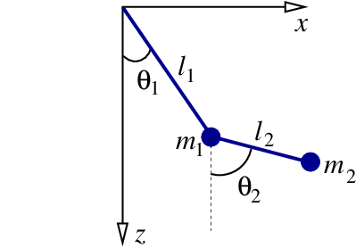
a) Show that the Lagrangian of the double pendulum is given by

\[ L = \frac{1}{2} (m_1 + m_2) \ell_1^2 \dot{\theta}_1^2 + \frac{1}{2} m_2 \ell_2^2 \dot{\theta}_2^2 + m_2 \ell_1 \ell_2 \dot{\theta}_1 \dot{\theta}_2 \cos(\theta_1 - \theta_2) + (m_1 + m_2) g\ell_1 \cos\theta_1 + m_2 g \ell_2 \cos\theta_2. \]

b) Calculate the generalized momenta $p_1$ and $p_2$ and express $\dot{\theta}_1$ and $\dot{\theta}_2$ in terms of them.

c) Find the Hamiltonian of the double pendulum.

d) Show that Hamilton's equations are

\begin{array} \dot{\theta}_1 &=& \frac{\ell_2 p_1 - \ell_1 p_2 \cos(\theta_1-\theta_2)}{\ell_1^2\ell_2 \bigl[ m_1 + m_2 \sin^2(\theta_1 - \theta_2) \bigr]}, \\ \dot{\theta}_1 &=& \frac{(m_1+m_2) \ell_1 p_2 - m_2 \ell_2 p_1 \cos(\theta_1-\theta_2)}{\ell_1\ell_2^2 \bigl[ m_1 + m_2 \sin^2(\theta_1 - \theta_2) \bigr]}, \\ \dot{p}_1 &=& -A + B - (m_1+m_2) g \ell_1 \sin\theta_1, \\ \dot{p}_2 &=& A - B - m_2 g \ell_2 \sin\theta_2, \end{array}

where

\[ A = \frac{p_1 p_2 \sin(\theta_1-\theta_2)}{\ell_1 \ell_2 \bigl[ m_1 + m_2 \sin^2(\theta_1 - \theta_2) \bigr]}\]

and

\[B = \frac{ m_2 \ell_2^2 p_1^2 + (m_1+m_2) \ell_1^2 p_2^2 - 2m_2 \ell_1 \ell_2 p_1 p_2 \cos(\theta_1-\theta_2)} {\ell_1^2 \ell_2^2 \bigl[ m_1 + m_2 \sin^2(\theta_1 - \theta_2) \bigr]^2} \sin(\theta_1-\theta_2) \cos(\theta_1 - \theta_2).\]

Chapter 3: Hamiltonian Mechanics

3.1 From Lagrange to Hamilton

3.1.1 Hamilton's Canonical Equations

3.1.2 Conservation Statements

3.1.3 Phase Space

3.1.4 Hamilton's Equations from Hamilton's Principle

3.2 Applications of Hamiltonian Mechanics

3.2.1 Canonical Equations in Cartesian Coordinates

3.2.2 Canonical Equations in Cylindrical Coordinates

3.2.3 Canonical Equations in Spherical Coordinates

3.2.4 Planar Pendulum

3.2.5 Spherical Pendulum

3.2.6 Rotating Pendulum

3.2.7 Rolling Disk

3.2.8 Kepler's Problem

3.2.9 Charged Particle in an Electromagnetic Field

3.3 Liouville's Theorem

3.3.1 Formulation of the Theorem

3.3.2 Case Study: Linear Pendulum

3.3.3 Proof of Liouvilles's

3.3.4 Poisson Brackets

3.4 Canonical Transformation

3.4.1 Introduction

3.4.2 Case Study: Linear Pendulum

3.4.3 General Theory of Canonical Transformations

3.4.4 Alternative Generating Functions

3.4.5 Direct Conditions

3.4.6 Canonical Invariants

3.5 Hamilton-Jacobi Equation

3.5.1 Action as a Function of the Coordinates and Time

3.5.2 Hamilton-Jacobi Equation

3.5.3 Case Study: Linear Pendulum

3.6 Problems

Department Resources

Administrative Links

Contact Us