Chapter 1: Newtonian Mechanics

Equations will not display properly in Safari-please use another browser

1.1 Reference frames

An important aspect of the fundamental law of Newtonian mechanics,

$$\begin{equation} \boldsymbol{F} = m \boldsymbol{a}, \tag{1.1.1} \end{equation}$$

is that it is formulated in a reference frame which is either at rest or moving with a uniform velocity (the velocity must be constant both in magnitude and in direction). Such frames are called inertial frames. A reference frame is a set of three axes attached to a point $O$ called the origin. The position of the origin in space is arbitrary, but some specific choices are sometimes convenient. For example, when describing a system of $N$ bodies it is usually a good idea to place the origin at the centre of mass (which will be introduced below). The origin of an inertial frame is either fixed or moving uniformly relative to another inertial frame. The orientation of the axes is also arbitrary, but some specific choices can again simplify the description. For example, when studying the motion of a particle in a gravitational field it is convenient to align one of the coordinate axes with the direction of the gravitational force.

The coordinate axes define a set of basis vectors $\boldsymbol{\hat{x}}$, $\boldsymbol{\hat{y}}$, and $\boldsymbol{\hat{z}}$. (These are sometimes denoted $\boldsymbol{i}$,$\boldsymbol{j}$, and $\boldsymbol{k}$.) These vectors point in the directions of increasing $x$, $y$, and $z$, respectively, and they all have a unit norm: $\boldsymbol{\hat{x}} \cdot \boldsymbol{\hat{x}} = \boldsymbol{\hat{y}} \cdot \boldsymbol{\hat{y}} = \boldsymbol{\hat{z}} \cdot \boldsymbol{\hat{z}} = 1$; this property is indicated by the ``hat'' notation. Relative to a choice of origin $O$, a particle has a position vector $\boldsymbol{r}(t)$ at time $t$. This is decomposed in the basis as

$$\begin{equation} \boldsymbol{r}(t) = x(t) \boldsymbol{\hat{x}} + y(t) \boldsymbol{\hat{y}} + z(t) \boldsymbol{\hat{z}}. \tag{1.1.2} \end{equation}$$

The functions $x(t)$, $y(t)$, and $z(t)$ are the particle's coordinates relative to the reference frame. The coordinates change as $t$ varies, and the particle traces a trajectory in three-dimensional space. The central goal of Newtonian mechanics is to determine this trajectory, assuming that the force $\boldsymbol{F}$ acting on the particle is known at all times.

The particle's velocity vector is

$$\begin{equation} \boldsymbol{v}(t) = \frac{d \boldsymbol{r}}{dt} = \dot{x}(t) \boldsymbol{\hat{x}} + \dot{y}(t) \boldsymbol{\hat{y}} + \dot{z}(t) \boldsymbol{\hat{z}}, \tag{1.1.3} \end{equation}$$

where we have introduced the notation $\dot{x} = dx/dt = v_x$; we shall also use $\boldsymbol{\dot{r}} = d\boldsymbol{r}/dt$ as an alternative notation for the vector $\boldsymbol{v}$. The particle's momentum vector is defined by

$$\begin{equation} \boldsymbol{p} = m \boldsymbol{v}, \tag{1.1.4} \end{equation}$$

where $m$ is the particle's mass. The particle's acceleration vector is

$$\begin{equation} \boldsymbol{a}(t) = \frac{d \boldsymbol{v}}{dt} = \ddot{x}(t) \boldsymbol{\hat{x}} + \ddot{y}(t) \boldsymbol{\hat{y}} + \ddot{z}(t) \boldsymbol{\hat{z}}, \tag{1.1.5} \end{equation}$$

with the notation $\ddot{x} = d^2x/dt^2 = \dot{v}_x = a_x$. Newton's equation, $m \boldsymbol{a} = \boldsymbol{F}$, has the mathematical structure of a system of second-order differential equations for the coordinates $x(t)$, $y(t)$, and $z(t)$. To describe the particle's trajectory, knowing the force, it is necessary to integrate these differential equations.

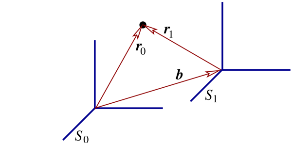
Suppose that we have two reference frames, $S_0$ and $S_1$, separated by a displacement $\boldsymbol{b}$ (see Fig.1.1). Relative to $S_1$ the position vector of a particle is $\boldsymbol{r}_1$; relative to $S_0$ it is $\boldsymbol{r}_0$. The transformation between the two position vectors is clearly $\boldsymbol{r}_0 = \boldsymbol{b} + \boldsymbol{r}_1$, or

$$\begin{equation} \boldsymbol{r}_1 = \boldsymbol{r}_0 - \boldsymbol{b}. \tag{1.1.6} \end{equation}$$

Suppose now that $S_1$ moves relative to $S_0$, so that the vector $\boldsymbol{b}$ depends on time. Since the position vectors also depend on time, Eq.(1.1.6) should be written as $\boldsymbol{r}_1(t) = \boldsymbol{r}_0(t) - \boldsymbol{b}(t)$. Taking a time derivative produces the transformation between the velocity vectors:

$$\begin{equation} \boldsymbol{v}_1 = \boldsymbol{v}_0 - \boldsymbol{\dot{b}}. \tag{1.1.7} \end{equation}$$

Taking a second time derivative gives us the transformation between the acceleration vectors:

$$\begin{equation} \boldsymbol{a}_1 = \boldsymbol{a}_0 - \boldsymbol{\ddot{b}}. \tag{1.1.8} \end{equation}$$

If $S_0$ is an inertial frame, then the equations of motion for the particle as viewed in $S_0$ are $m \boldsymbol{a}_0 = \boldsymbol{F}$. In $S_1$ the equations are instead

$$\begin{equation} m \boldsymbol{a}_1 = \boldsymbol{F} - m \boldsymbol{\ddot{b}}. \tag{1.1.9} \end{equation}$$

We see that Newton's equation is preserved only if $\boldsymbol{\ddot{b}} = \boldsymbol{0}$, that is, if $\boldsymbol{\dot{b}}$ is a constant vector. In this case $S_1$ moves relative to $S_0$ with a constant velocity, and it is also an inertial frame. When, however, $S_1$ is not inertial, the equations of motion do not take the Newtonian form. We have instead Eq.~($\ref{1.1.9}$), which can be rewritten as

$$m \boldsymbol{a}_1 = \boldsymbol{F} + \boldsymbol{F}_{\rm fictitious},$$

with $\boldsymbol{F}_{\rm fictitious} = -m \boldsymbol{\ddot{b}}$. The second term on the right can be thought of as a fictitious force that arises from the fact that the reference frame is not inertial. A well-known example is the centrifugal force, which arises in a rotating (and therefore non-inertial) frame of reference.

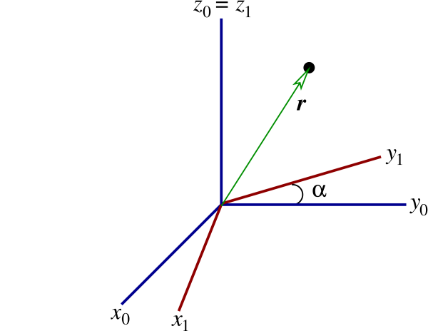
We now consider a situation in which $S_1$ and $S_0$ are both inertial. We assume, in fact, that they share a common origin $O$, but that they differ in the orientation of the coordinate axes. A concrete example (see Fig.1.2) is one in which $S_1$ is obtained from $S_0$ by a rotation around the $z$ axis. In this case the basis vectors $\boldsymbol{\hat{x}_1}$ and $\boldsymbol{\hat{y}_1}$ differ in direction from $\boldsymbol{\hat{x}_0}$ and $\boldsymbol{\hat{y}_0}$. Similarly, the particle's coordinates $x_1(t)$ and $y_1(t)$ differ from $x_0(t)$ and $y_0(t)$. But it is an important fact that the position vector $\boldsymbol{r}(t)$ is not affected by the rotation:

$$\begin{align} \boldsymbol{r}_1 &= x_1 \boldsymbol{\hat{x}_1} + y_1 \boldsymbol{\hat{y}_1} + z_1 \boldsymbol{\hat{z}_1} \\ &= x_0 \boldsymbol{\hat{x}_0} + y_0 \boldsymbol{\hat{y}_0}+z_0 \boldsymbol{\hat{z}_0} \\ &= \boldsymbol{r}_0. \end{align}$$

This conclusion follows simply from the fact that $\boldsymbol{r} = \boldsymbol{r}_1 = \boldsymbol{r}_0$ is a vector which points from $O$ to the particle, independently of the orientation of the reference frame. So although the basis vectors and the coordinates all change separately under a rotation of the frame, the position vector is invariant. From this observation it follows that $\boldsymbol{v}_1 = \boldsymbol{v}_0 = \boldsymbol{v}$ and $\boldsymbol{a}_1 = \boldsymbol{a}_0 = \boldsymbol{a}$: the velocity and acceleration vectors also are invariant under a rotation of the reference frame. Similar considerations reveal that the vector $\boldsymbol{F}$ is invariant, and we conclude that the form of Newton's equation $\boldsymbol{F} = m \boldsymbol{a}$ is not affected by a rotation of the reference frame. (These invariance properties are exactly what motived the formulation of Newton's mechanics in terms of vectorial quantities.)

---

Exercise 1.1: Determine how the coordinates $x$ and $y$, as well as the basis vectors $\boldsymbol{\hat{x}}$ and $\boldsymbol{\hat{y}}$, change under a rotation around the $z$ axis by an angle $\alpha$. Then show mathematically that $\boldsymbol{r}$ is invariant under the transformation.

---

1.2 Alternative Coordinate System

The discussion of the previous section will have made it clear that the Cartesian coordinates $(x,y,z)$ play an important role in Newtonian mechanics. We might even say that they have a preferred status. The same can be said of the associated set of basis vectors $\boldsymbol{\hat{x}}$, $\boldsymbol{\hat{y}}$, and $\boldsymbol{\hat{z}}$. We are aware, however, of situations in which it may be advantageous not to use the Cartesian coordinates, but to switch to another, more convenient system. What happens then to the formulation of our fundamental law, $\boldsymbol{F} = m\boldsymbol{a}$? The answer, as we shall see in this section, is that while the law itself does not change, its concrete mathematical form may actually look very different.

To keep things specific we choose here to work in the $x$-$y$ plane (we set $z = 0$) and to consider a specific example of an alternative coordinate system, the polar coordinates $r$ and $\phi$. These are defined by

$$\begin{equation} x = r \cos\phi, \qquad y = r \sin\phi; \tag{1.2.1} \end{equation}$$

the radial coordinate $r$ measures the distance from the origin to the particle, and $\phi$ is the angle relative to the $x$ axis. In terms of the new coordinates the position vector is

$$\begin{equation} \boldsymbol{r} = (r\cos\phi) \boldsymbol{\hat{x}} + (r\sin\phi) \boldsymbol{\hat{y}}, \tag{1.2.2} \end{equation}$$

and it is now a function of $r$ and $\phi$. We may express this as $\boldsymbol{r} = \boldsymbol{r}(r,\phi)$, and the vector $\boldsymbol{r}$ points to the position identified by the coordinates $(r,\phi)$. Notice that $r$ is the magnitude of the position vector: $\boldsymbol{r} \cdot \boldsymbol{r} = r^2$.

As the particle moves in the plane its coordinates $r$ and $\phi$ vary with time, and the particle's velocity vector is $\boldsymbol{v} = \boldsymbol{\dot{r}}$, or

$$\begin{equation} \boldsymbol{v} = (\dot{r} \cos\phi - r \dot{\phi} \sin\phi) \boldsymbol{\hat{x}} + (\dot{r} \sin\phi + r \dot{\phi} \cos\phi) \boldsymbol{\hat{y}}. \tag{1.2.3} \end{equation}$$

Notice that the magnitude of the velocity vector is {\it not equal} to $\dot{r}$; instead $\boldsymbol{v} \cdot \boldsymbol{v} = \dot{r}^2 + r^2 \dot{\phi}^2$. The acceleration vector is then $\boldsymbol{a} = \boldsymbol{\dot{v}}$, or

$$\begin{align} \boldsymbol{a} &= (\ddot{r} \cos\phi - 2 \dot{r}\dot{\phi} \sin\phi - r\dot{\phi}^2 \cos\phi - r\ddot{\phi} \sin\phi) \boldsymbol{\hat{x}} \nonumber + (\ddot{r} \sin\phi + 2 \dot{r}\dot{\phi} \cos\phi - r\dot{\phi}^2 \sin\phi + r\ddot{\phi} \cos\phi) \boldsymbol{\hat{y}}. \tag{1.2.4} \end{align}$$

As presented here, these vectors are resolved in the Cartesian basis $\boldsymbol{\hat{x}}$ and $\boldsymbol{\hat{y}}$. It is more convenient to resolve them instead in the polar basis $\boldsymbol{\hat{r}}$ and $\boldsymbol{\hat{\phi}}$, where

$$\begin{equation} \boldsymbol{\hat{r}} = \text{unit vector pointing in the direction of increasing $r$} \tag{1.2.5} \end{equation}$$

and

$$\begin{equation} \boldsymbol{\hat{\phi}} = \text{unit vector pointing in the direction of increasing $\phi$}. \tag{1.2.6} \end{equation}$$

It is important to note that these new basis vectors, unlike $\boldsymbol{\hat{x}}$ and $\boldsymbol{\hat{y}}$, are not constant vectors: their directions change as we move from point to point in the plane.

To find an expression for $\boldsymbol{\hat{r}}$ we observe that by construction, the infinitesimal vector

$$\delta \boldsymbol{r} \equiv \boldsymbol{r}(r+\delta r,\phi) - \boldsymbol{r}(r,\phi) = \frac{\partial \boldsymbol{r}}{\partial r}\, \delta r$$

points in the direction of increasing $r$. This means that $\boldsymbol{\hat{r}}$ must be proportional to $\partial \boldsymbol{r}/\partial r$. Looking back at Eq.(1.2.2), we see that this is given by $\cos\phi\, \boldsymbol{\hat{x}} + \sin\phi\, \boldsymbol{\hat{y}}$, and we find that this vector already has a unit norm: $(\partial \boldsymbol{r}/\partial r) \cdot (\partial \boldsymbol{r}/\partial r) = \cos^2\phi + \sin^2\phi = 1$. We conclude that

$$\begin{equation} \boldsymbol{\hat{r}} = \frac{\partial \boldsymbol{r}}{\partial r} = \cos\phi\, \boldsymbol{\hat{x}} + \sin\phi\, \boldsymbol{\hat{y}} \tag{1.2.7} \end{equation}$$

is the desired basis vector. We proceed similarly to find an expression for $\boldsymbol{\hat{\phi}}$. We observe that the infinitesimal vector

$$\delta \boldsymbol{r} \equiv \boldsymbol{r}(r,\phi+\delta \phi) - \boldsymbol{r}(r,\phi) = \frac{\partial \boldsymbol{r}}{\partial \phi}\, \delta \phi$$

points in the direction of increasing $\phi$. (Be careful: this is a different $\delta \boldsymbol{r}$ from the one considered before!) This means that $\boldsymbol{\hat{\phi}}$ must be proportional to $\partial \boldsymbol{r}/\partial \phi$, which is given by $-r\sin\phi\, \boldsymbol{\hat{x}} + r\cos\phi\, \boldsymbol{\hat{y}}$. The squared norm of this vector is $(\partial \boldsymbol{r}/\partial \phi) \cdot (\partial \boldsymbol{r}/\partial \phi) = r^2\sin^2\phi + r^2\cos^2\phi = r^2$, and to get a unit vector we must divide $\partial \boldsymbol{r}/\partial \phi$ by $r$. We conclude that

$$\begin{equation} \boldsymbol{\hat{\phi}} = \frac{1}{r} \frac{\partial \boldsymbol{r}}{\partial \phi} = -\sin\phi\, \boldsymbol{\hat{x}} + \cos\phi\, \boldsymbol{\hat{y}} \tag{1.2.8} \end{equation}$$

---

Exercise 1.2: Check that $\boldsymbol{\hat{r}} \cdot \boldsymbol{\hat{\phi}} = 0$.

---

Let us now work out the components of the vectors $\boldsymbol{r}$, $\boldsymbol{v}$, and $\boldsymbol{a}$ in the basis $(\boldsymbol{\hat{r}}, \boldsymbol{\hat{\phi}})$. According to Eqs.(1.2.2) and (1.2.7) we have

$$\begin{align} \boldsymbol{r} \cdot \boldsymbol{\hat{r}} &= \bigl[ (r\cos\phi) \boldsymbol{\hat{x}} + (r\sin\phi) \boldsymbol{\hat{y}} \bigr] \cdot \bigl[\cos\phi\, \boldsymbol{\hat{x}} + \sin\phi\, \boldsymbol{\hat{y}} \bigr] \\ &= r\cos^2\phi + r\sin^2\phi \\ &= r. \end{align}$$

Similarly, Eqs.(1.2.2) and (1.2.8) give

$$\begin{align} \boldsymbol{r} \cdot \boldsymbol{\hat{\phi}} &= \bigl[ (r\cos\phi) \boldsymbol{\hat{x}} + (r\sin\phi) \boldsymbol{\hat{y}} \bigr] \cdot \bigl[ -\sin\phi\, \boldsymbol{\hat{x}} + \cos\phi\, \boldsymbol{\hat{y}} \bigr] \\ &= -r\sin\phi \cos\phi + r\sin\phi\cos\phi \\ &= 0. \end{align}$$

From these results we infer that

$$\begin{equation} \boldsymbol{r} = r\, \boldsymbol{\hat{r}}, \tag{1.2.9} \end{equation}$$

and this expression should not come as a surprise, given the meaning of the quantities involved. Proceeding similarly with the vectors $\boldsymbol{v}$ and $\boldsymbol{a}$, we find that they are decomposed as

\begin{equation} \boldsymbol{v} = \dot{r}\, \boldsymbol{\hat{r}} + r\dot{\phi}\, \boldsymbol{\hat{\phi}} \tag{1.2.10}

and

$$\begin{equation} \boldsymbol{a} = \bigl( \ddot{r} - r \dot{\phi}^2 \bigr) \boldsymbol{\hat{r}} + \frac{1}{r} \frac{d}{dt} \bigl( r^2 \dot{\phi} \bigr) \boldsymbol{\hat{\phi}} \tag{1.2.11} \end{equation}$$

in the new basis. As we have pointed out, the components of $\boldsymbol{r}$ in the polar basis are obvious, and the components of $\boldsymbol{v}$ also can be understood easily: The radial component of the velocity vector must clearly be $v_r = \dot{r}$, and the tangential component must be $v_\phi = r \dot{\phi}$ because the factor of $r$ converts the angular velocity $\dot{\phi}$ into a linear velocity.

The components of the acceleration vector are not so easy to interpret. It is important to notice that the radial component of the acceleration vector is not simply $a_r = \ddot{r}$, and the angular component is not simply $a_\phi = \ddot{\phi}$. It is a general observation that the components of the acceleration vector are not simple in nonCartesian coordinate systems. It should be observed that the radial component of the acceleration vector contains both a radial part $\ddot{r}$ and a centrifugal part $-r\dot{\phi}^2 = -v_\phi^2/r$.

---

Exercise 1.3: Verify by explicit calculation that Eqs.(1.2.10) and (1.2.11) are correct.

---

Suppose now that the force $\boldsymbol{F}$ has been resolved in the polar basis ($\boldsymbol{\hat{r}}$, $\boldsymbol{\hat{\phi}}$). We have

$$\begin{equation} \boldsymbol{F} = F_r \boldsymbol{\hat{r}} + F_\phi \boldsymbol{\hat{\phi}}, \tag{1.2.12} \end{equation}$$

and Newton's law $\boldsymbol{F} = m \boldsymbol{a}$ breaks down into two separate equations, the radial component

$$\begin{equation} \ddot{r} - r \dot{\phi}^2 = \frac{F_r}{m} \tag{1.2.13} \end{equation}$$

and the angular component

$$\begin{equation} \frac{d}{dt} \bigl( r^2 \dot{\phi} \bigr) = \frac{r F_\phi}{m}. \tag{1.2.14} \end{equation}$$

These are the equations of motion for a particle subjected to a force $\boldsymbol{F}$, expressed in polar coordinates $(r,\phi)$. When, for example, $F_\phi = 0$ and the force is purely radial, then according to Eq.(1.2.14), $r^2 \dot{\phi} = r v_\phi$ is a constant of the motion. When, in addition, $\ddot{r} = 0$ and the particle travels on a circle $r = \text{constant}$, then Eq.(1.2.13) reduces to $r \dot{\phi}^2 = v_\phi^2/r = -F_r/m$; this is the familiar equality between the centrifugal acceleration $v_\phi^2/r$ and (minus) the radial component of the force (divided by the mass).

---

Exercise 1.4: Consider the spherical coordinates $(r,\theta,\phi)$ defined by $x = r\sin\theta\cos\phi$, $y = r\sin\theta\sin\phi$, and $z = r\cos\theta$. Show that in this alternative coordinate system, the basis vectors are given by $$\begin{align} \boldsymbol{\hat{r}} &= \frac{\partial \boldsymbol{r}}{\partial r} = \sin\theta\cos\phi\, \boldsymbol{\hat{x}} + \sin\theta\sin\phi \boldsymbol{\hat{y}} + \cos\theta\, \boldsymbol{\hat{z}}, \\ \boldsymbol{\hat{\theta}} &= \frac{1}{r}\frac{\partial \boldsymbol{r}}{\partial \theta} = \cos\theta\cos\phi\, \boldsymbol{\hat{x}} + \cos\theta\sin\phi \boldsymbol{\hat{y}} - \sin\theta\, \boldsymbol{\hat{z}}, \\ \boldsymbol{\hat{\phi}} &= \frac{1}{r\sin\theta} \frac{\partial \boldsymbol{r}}{\partial \phi} = -\sin\phi\, \boldsymbol{\hat{x}} + \cos\phi \boldsymbol{\hat{y}}. \end{align}$$ Verify that these vectors are all orthogonal to each other.

---

1.3 Mechanics of a Single Body

In this section we explore some consequences of the law $\boldsymbol{F} = m \boldsymbol{a}$ when it applies to a single particle.

1.3.1 Line Integrals

We begin with a review of some relevant mathematics. Let $\boldsymbol{A}$ be a vector field in three-dimensional space. (A vector field is a vector that is defined in a region of space and which may vary from position to position in that region.) Let $C$ be a curve in three-dimensional space, and let $d\boldsymbol{s}$ be the displacement vector along the curve. The displacement vector is defined so that $d\boldsymbol{s}$ is everywhere tangent to the curve, and such that its norm $ds = |d\boldsymbol{s}|$ is equal to the distance between two neighbouring points on the curve; the total length of the curve is the integral $\int_C ds$. Now introduce

$$\int_1^2 \boldsymbol{A} \cdot d\boldsymbol{s},$$

the line integral of the vector field $\boldsymbol{A}$ between point 1 and point 2 on the curve $C$. Such integrals occur often in physics. In the present context the force $\boldsymbol{F}$ will play the role of the vector field $\boldsymbol{A}$, and the particle's trajectory will play the role of the curve $C$; we then have $d\boldsymbol{s} = d\boldsymbol{r} = \boldsymbol{v} dt$ and the line integral will be the work done by the force as the particle moves from point 1 to point 2.

It is a fundamental theorem of vector calculus that if a line integral between two fixed points in space does not depend on the curve joining the points, then the vector field $\boldsymbol{A}$ must be the gradient $\boldsymbol{\nabla} f$ of some scalar function $f$. This theorem is essentially a consequence of the identity

$$\int_1^2 \boldsymbol{\nabla} f \cdot d\boldsymbol{s} = \int_1^2 \frac{df}{ds}\, ds = f(2) - f(1) \quad \text{independently of the curve},$$

which is a generalization of the statement $\int_a^b (df/dx)\, dx = f(b) - f(a)$ from ordinary calculus. Another way of presenting this result is to say that if $\boldsymbol{A} = \boldsymbol{\nabla} f$, then $\oint \boldsymbol{A} \cdot d\boldsymbol{s} = 0$ for any closed curve $C$ in three-dimensional space. This last statement follows because if the curve $C$ is closed, point 2 is identified with point 1, and $\oint \boldsymbol{\nabla} f \cdot d\boldsymbol{s} = f(1) - f(1) = 0$.

To illustrate these notions let us work through a concrete example. Consider the vector field $\boldsymbol{A} = (x,y)$ in two-dimensional space. We wish first to evaluate the line integral of $\boldsymbol{A}$ along the $x$ axis, from $x = -1$ to $x = +1$ (see Fig.1.3). The safest way to proceed is to first obtain a parametric description of the curve $C$, which in this case is the line segment that links the points $x = \mp 1$. We may describe this curve in the following way:

$$x(u) = -1 + 2u, \qquad y(u) = 0,$$

where the parameter $u$ is restricted to the interval $0 \leq u \leq 1$. (The choice of parameterization is arbitrary; we might just as well have chosen $x$ as the parameter, but it is generally a good idea to keep the parameter distinct from the coordinates.) From these equations it follows that the displacement vector on $C$ has the components $dx = 2\, du$ and $dy = 0$, so that $d\boldsymbol{s} = (2\, du, 0)$. The vector field evaluated on $C$ is $\boldsymbol{A} = (-1 + 2u, 0)$, and we have $\boldsymbol{A} \cdot d\boldsymbol{s} = 2(-1 + 2u)\, du$. The line integral is then

$$\int_C \boldsymbol{A} \cdot d\boldsymbol{s} = \int_0^1 2(-1+2u)\, du.$$

Evaluating this ordinary integral is straightforward, and the result is zero. We therefore have

$$\int_C \boldsymbol{A} \cdot d\boldsymbol{s} = 0$$

for this choice of curve linking the points $(x=-1,y=0)$ and $(x=1,y=0)$.

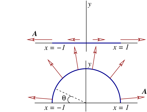
Let us now evaluate the line integral of $\boldsymbol{A}$ along a different curve $C'$ which joins the same two endpoints (refer again to Fig.1.3); we choose for $C'$ a semi-circle of unit radius, which we describe by the parametric relations

$$x(\theta) = -\cos\theta, \qquad y(\theta) = \sin\theta,$$

with a parameter $\theta$ running from $\theta = 0$ to $\theta = \pi$. Now we have $dx = \sin\theta\, d\theta$, $dy = \cos\theta\, d\theta$, and the displacement vector on $C'$ is $d\boldsymbol{s} = (\sin\theta\, d\theta, \cos\theta\, d\theta)$. The vector field evaluated on $C'$ is $\boldsymbol{A} = (-\cos\theta,\sin\theta)$, and we have $\boldsymbol{A} \cdot d\boldsymbol{s} = 0$. The line integral is obviously

$$\int_{C'} \boldsymbol{A} \cdot d\boldsymbol{s} = 0$$

for this choice of curve also. You might experiment with other curves, and invariably you will find that $\int \boldsymbol{A} \cdot d\boldsymbol{s} = 0$ for all curves $C$ that link the points $(-1,0)$ and $(1,0)$ in the $x$-$y$ plane.

---

Exercise 1.5: Evaluate the line integral $\int_{C''} \boldsymbol{A} \cdot d\boldsymbol{s}$ for the vector field $\boldsymbol{A} = (x,y)$, for a curve $C''$ that consists of a line segment that goes from $(-1,0)$ to $(0,-1)$ and another line segment that goes from $(0,-1)$ to $(1,0)$.

---

Because the line integral is independent of the path, $\boldsymbol{A}$ must be the gradient of a scalar function $f$. We must have $A_x = \partial f/\partial x = x$ and $A_y = \partial f/\partial y = y$. Integrating the first equation gives

$$f = \frac{1}{2} x^2 + \text{unknown function of $y$},$$

where we indicate that the ``constant of integration'' can in fact depend on $y$, which is held fixed during integration with respect to $x$. Integrating instead the second equation gives

$$f = \frac{1}{2} y^2 + \text{unknown function of $x$}.$$

These results are compatible only if the unknown function of $y$ is in fact $\frac{1}{2} y^2$, and the unknown function of $x$ is $\frac{1}{2} x^2$. We may still add a true constant to the result, and we find that the function $f$ must be given by

$$f = \frac{1}{2} \bigl( x^2 + y^2 \bigr) + f_0,$$

where $f_0 = \text{constant}$. It is then easy to verify that $\boldsymbol{\nabla} f = \boldsymbol{A}$. It now becomes clear why the line integral had to be zero for any path linking the points $(-1,0)$ and $(1,0)$: Irrespective of the path the integral has to be equal to $f(1,0) - f(-1,0) = (\frac{1}{2} + f_0) - (\frac{1}{2} + f_0) = 0$, as we have found for $C$ and $C'$.

1.3.2 Conservation of Linear Momentum

We now proceed with our exploration of the consequences of the dynamical law $\boldsymbol{F} = m \boldsymbol{a}$. The first main consequence follows immediately from Newton's equation: In the absence of a force acting on the particle, the linear momentum $\boldsymbol{p} = m \boldsymbol{v}$ is a constant vector. This follows from the alternative expression of Newton's law,

$$\begin{equation} \boldsymbol{F} = \frac{d \boldsymbol{p}}{dt}; \tag{1.3.1} \end{equation}$$

if $\boldsymbol{F} = \boldsymbol{0}$ then $d\boldsymbol{p}/dt = \boldsymbol{0}$ and the vector $\boldsymbol{p}$ must be constant. We therefore have conservation of (linear) momentum in the absence of an applied force.

1.3.3 Conservation of Angular Momentum

Relative to a choice of origin $O$, the angular momentum of a particle at position $\boldsymbol{r}$ is defined by

$$\begin{equation} \boldsymbol{L} = \boldsymbol{r} \times \boldsymbol{p} = m \boldsymbol{r} \times \boldsymbol{v}. \tag{1.3.2} \end{equation}$$

The angular-momentum vector changes if the origin of the reference frame is shifted to a different point in space. The torque acting on the particle is defined by

$$\begin{equation} \boldsymbol{N} = \boldsymbol{r} \times \boldsymbol{F}. \tag{1.3.3} \end{equation}$$

(This is also called the moment of force.) We have, as a consequence of Newton's equation, $d\boldsymbol{L}/dt = m ( \boldsymbol{v} \times \boldsymbol{v} + \boldsymbol{r} \times \boldsymbol{a} ) = \boldsymbol{r} \times \boldsymbol{F}$, since the first term obviously vanishes. This gives

$$\begin{equation} \frac{d\boldsymbol{L}}{dt} = \boldsymbol{N}, \tag{1.3.4} \end{equation}$$

and we obtain a statement of angular-momentum conservation: In the absence of a torque acting on the particle, the angular momentum $\boldsymbol{L}$ is a constant vector. It is clear that $\boldsymbol{N} = \boldsymbol{0}$ when $\boldsymbol{F} = \boldsymbol{0}$, but it is possible to have a vanishing torque even when $\boldsymbol{F} \neq \boldsymbol{0}$; this occurs when $\boldsymbol{F}$ always points in the direction of $\boldsymbol{r}$.

1.3.4 Conservation of Energy

The statements of conservation of linear and angular momenta were easy to formulate and prove, but these statements hold only in very rare circumstances: $\boldsymbol{F}$ must vanish for $\boldsymbol{p}$ to be constant, and $\boldsymbol{N}$ must vanish for $\boldsymbol{L}$ to be constant. As we shall see, the statement of conservation of energy is more difficult to make, but it holds much more widely.

Let a particle move from point 1 to point 2 under the action of a force $\boldsymbol{F}$. The total work done on the particle by the force, as it moves from 1 to 2, is by definition the line integral

$$\begin{equation} W_{12} = \int_1^2 \boldsymbol{F} \cdot d\boldsymbol{r}, \tag{1.3.5} \end{equation}$$

where $d\boldsymbol{r} = \boldsymbol{v}\, dt$ is the displacement vector along the particle's trajectory. As we shall now infer, the line integral is equal to the total change in the particle's kinetic energy,

$$\begin{equation} T = \frac{1}{2} m v^2 = \text{kinetic energy}, \tag{1.3.6} \end{equation}$$

as it moves from 1 to 2. We have introduced the notation $v^2 = \boldsymbol{v} \cdot \boldsymbol{v} = |\boldsymbol{v}|^2$. The statement of the work-energy theorem is thus

$$\begin{equation} W_{12} = T(2) - T(1). \tag{1.3.7} \end{equation}$$

To prove this we substitute $\boldsymbol{F} = m d\boldsymbol{v}/dt$ and $d\boldsymbol{r} = \boldsymbol{v}\, dt$ inside the line integral of Eq.(1.3.5). We get

$$W_{12} = m \int_1^2 \frac{d \boldsymbol{v}}{dt} \cdot \boldsymbol{v}\, dt.$$

The integrand is

$$\begin{align} \frac{d \boldsymbol{v}}{dt} \cdot \boldsymbol{v} &= \frac{d v_x}{dt} v_x + \frac{d v_y}{dt} v_y + \frac{d v_x}{dt} v_y \\ &= \frac{1}{2} \frac{d}{dt} v_x^2 + \frac{1}{2} \frac{d}{dt} v_y^2 + \frac{1}{2} \frac{d}{dt} v_z^2 \\ &=  \frac{1}{2} \frac{d}{dt} \biggl( v_x^2 + v_y^2 + v_z^2 \biggr) \\ &= \frac{d}{dt} \biggl( \frac{1}{2} v^2 \biggr), \end{align}$$

and the line integral becomes

$$W_{12} = \int_1^2 \frac{d}{dt} \biggl( \frac{1}{2} m v^2 \biggr)\, dt = \int_1^2 \frac{dT}{dt}\, dt = \int_1^2 dT = T(2) - T(1).$$

This is the same statement as in Eq.(1.3.7), and we have established the work-energy theorem.

In very many situations the line integral $\int_1^2 \boldsymbol{F} \cdot d\boldsymbol{r}$ is actually independent of the trajectory adopted by the particle to go from point 1 to point 2. In these situations we must have that $\boldsymbol{F}$ is the gradient of some scalar function $f(\boldsymbol{r})$. We write $f = -V$, inserting a minus sign for reasons of convention, and express the force as

$$\begin{equation} \boldsymbol{F} = -\boldsymbol{\nabla} V(\boldsymbol{r}). \tag{1.3.8} \end{equation}$$

The scalar function $V$ is known as the potential energy of the particle. When $\boldsymbol{F}$ is expressed as in Eq.(1.3.8) the line integral of Eq.(1.3.5) becomes

$$W_{12} = -\int_1^2 \boldsymbol{\nabla} V \cdot d\boldsymbol{r} = -\bigl[ V(2) - V(1) \bigr],$$

and this is clearly independent of the particle's trajectory: The total work done is equal to the difference $V(1) - V(2)$ no matter how the particle moves from 1 to 2. Equation (1.3.7) then becomes $V(1) - V(2) = T(2) - T(1)$, or $T(1) + V(1) = T(2) + V(2)$. This tells us that the quantity $T + V$ stays constant as the particle moves from point 1 to point 2. We therefore have obtained the statement of conservation of total mechanical energy

$$\begin{equation} E = T + V = \frac{1}{2} m v^2 + V(\boldsymbol{r}) \tag{1.3.9} \end{equation}$$

for a particle moving under the action of a force $\boldsymbol{F}$ that derives from a potential $V$.

We can verify directly from Eq.(1.3.9) that the total energy is a constant of the motion. We have

$$\frac{dE}{dt} = \frac{1}{2} m \frac{dv^2}{dt} + \frac{dV}{dt}.$$

As we have seen,

$$\frac{dv^2}{dt} = 2 \frac{d\boldsymbol{v}}{dt} \cdot \boldsymbol{v}.$$

The potential energy $V$ depends on time only through the changing position of the particle: $V = V(\boldsymbol{r}(t)) = V(x(t),y(t),z(t))$. We therefore have

$$\begin{align} \frac{dV}{dt} &= \frac{\partial V}{\partial x} \frac{dx}{dt} + \frac{\partial V}{\partial y} \frac{dy}{dt} + \frac{\partial V}{\partial z} \frac{dz}{dt} \\ &= \boldsymbol{\nabla} V \cdot \boldsymbol{v}. \end{align}$$

All of this gives

$$\begin{align} \frac{dE}{dt} &= m \boldsymbol{a} \cdot \boldsymbol{v} + \boldsymbol{\nabla} V \cdot\boldsymbol{v} \\ &= \boldsymbol{F} \cdot \boldsymbol{v} - \boldsymbol{F} \cdot \boldsymbol{v} \\ &= 0, \end{align}$$

as expected.

An example of a force that derives from a potential is gravity: The force

$$\begin{equation} \boldsymbol{F}_{\rm gravity} = m \boldsymbol{g} = mg (0,0,-1) \tag{1.3.10} \end{equation}$$

is the negative gradient of

$$\begin{equation} V_{\rm gravity} = m g z. \tag{1.3.11} \end{equation}$$

We have indicated that the vector $\boldsymbol{g}$ points in the negative $z$ direction (down, that is); its magnitude is the gravitational acceleration $g \simeq 9.8\ \text{m}/\text{s}^2$. The total mechanical energy $E$ is conserved when a particle moves under the action of the gravitational force.

An example of a force that does <em>not</em> derive from a potential is the frictional force

$$\begin{equation} \boldsymbol{F}_{\rm friction} = - k \boldsymbol{v}, \tag{1.3.12} \end{equation}$$

where $k > 0$ is the coefficient of friction; this force acts in the direction opposite to the particle's motion and exerts a drag. It is indeed easy to see that $\boldsymbol{F}_{\rm friction}$ cannot be expressed as the gradient of a function of $\boldsymbol{r}$. (The expression $V_{\rm friction} = k \boldsymbol{v} \cdot \boldsymbol{r}$ might seem to work, but this potential depends on both $\boldsymbol{r}$ and $\boldsymbol{v}$, and this is not allowed.) This implies that in the presence of a frictional force, the total mechanical energy of a particle is not conserved. The reason is that the friction produces heat, which is rapidly dissipated away; because this heat comes at the expense of the particle's mechanical energy, $E$ cannot be conserved. Energy conservation as a whole, of course, applies: the amount by which $E$ decreases matches the amount of heat dissipated into the environment.

It is important to understand that the work-energy theorem of Eq.(1.3.7) is always true, whether or not the force $\boldsymbol{F}$ derives from a potential. But whether $E$ is conserved or not depends on this last property: When $\boldsymbol{F} = -\boldsymbol{\nabla} V$ we have $dE/dt = 0$ and the total mechanical energy is conserved; but $E$ is not in general conserved when the force does not derive from a potential.

1.3.5 Case Study #1: Particle in a Gravitational Field

To illustrate the formalism presented in the preceding subsections we now review the problem of determining the motion of a particle in a gravitational field. The force is given by Eq.(1.3.10), $\boldsymbol{F} = m\boldsymbol{g} = mg(0,0,-1)$, and the potential by Eq.(1.3.11), $V = m g z$. The equations of motion are

$$\begin{equation} \ddot{x} = 0, \qquad \ddot{y} = 0, \qquad \ddot{z} = -g. \tag{1.3.13} \end{equation}$$

These are easily integrated:

$$\begin{equation} x(t) = x(0) + v_x(0) t, \qquad y(t) = y(0) + v_y(0) t, \qquad z(t) = z(0) + v_z(0) t - \frac{1}{2} g t^2. \tag{1.3.14} \end{equation}$$

These equations describe parabolic motion. Here $x(0), y(0), z(0)$ are the positions at time $t=0$, and $v_x(0)$, $v_y(0)$, and $v_z(0)$ are the components of the velocity vector at $t=0$; these quantities are the initial conditions that must be specified in order for the motion to be uniquely known at all times. The velocity vector at time $t$ is obtained by differentiating Eqs.(1.3.14); we get

$$\begin{equation} v_x(t) = v_x(0), \qquad v_y(t) = v_y(0), \qquad v_z(t) = v_z(0) - g t. \tag{1.3.15} \end{equation}$$

With Eqs.(1.3.14) and (1.3.15) we have sufficient information to compute the total mechanical energy $E = T + V$ of the particle. After some simple algebra we obtain

$$\begin{equation} E = \frac{1}{2} m \Bigl[ v_x(0)^2 + v_y(0)^2 + v_z(0)^2 \bigr] + m g z(0) \tag{1.3.16} \end{equation}$$

for all times $t$; this is clearly a constant of the motion.

---

Exercise 1.6: Verify that Eqs.(1.3.14) really give the solution to the equations of motion $\boldsymbol{\ddot{r}} = \boldsymbol{g}$. Then compute $E$ and make sure that your result agrees with Eq.(1.3.16).

---

1.3.6 Case Study #2: Particle in a Gravitational Field Subjected to Air Resistance

We now suppose that the particle is subjected to both a gravitational force $m \boldsymbol{g}$ and a frictional force $-k \boldsymbol{v}$ supplied by the ambient air. For convenience we set $k = m/\tau$, thereby defining the quantity $\tau$, and the total applied force is

$$\begin{equation} \boldsymbol{F} = m( \boldsymbol{g} - \boldsymbol{v}/\tau ). \tag{1.3.17} \end{equation}$$

The equations of motion are $m \boldsymbol{a} = \boldsymbol{F}$, or $\boldsymbol{a} = \boldsymbol{g} - \boldsymbol{v}/\tau$, or again

$$\begin{equation} \boldsymbol{\ddot{r}} + \boldsymbol{\dot{r}}/\tau = \boldsymbol{g}. \tag{1.3.18} \end{equation}$$

We assume that the particle is released from a height $h$ with a zero initial velocity. The initial conditions are therefore $z(0) = h$ and $\dot{z}(0) = 0$. We assume also, for simplicity, that there is no motion in the $x$ and $y$ directions. The only relevant component of Eq.(1.3.18) is therefore

$$\begin{equation} \dot{v} + v/\tau = -g, \tag{1.3.19} \end{equation}$$

where we have set $v = \dot{z}$. To arrive at Eq.(1.3.19) we have used the fact that $\boldsymbol{g} = g(0,0,-1)$.

Our task is to solve the first-order differential equation of Eq.(1.3.19). We use the method of variation of parameters. Suppose first that $g = 0$. In this case the equation becomes $dv/dt = -v/\tau$ or $dv/v = -dt/\tau$. This is easily integrated, and we get $\ln(v/c) = -t/\tau$, or $v = c\, e^{-t/\tau}$. This is the solution for $g = 0$, and the constant of integration $c$ is the solution's parameter. To handle the case $g \neq 0$ we allow $c$ to depend on time --- we vary the parameter --- and we substitute the trial solution

$$v(t) = c(t) e^{-t/\tau}$$

into Eq.(1.3.19). We have $\dot{v} = \dot{c} e^{-t/\tau} - v/\tau$ and $-g = \dot{v} + v/\tau = \dot{c} e^{-t/\tau}$. The differential equation for $c(t)$ is therefore

$$\dot{c} = -g e^{t/\tau},$$

so that

$$c(t) = -g \tau e^{t/\tau} + c_0,$$

where $c_0$ is a true constant of integration. The result for $v(t)$ is then

$$v(t) = -g \tau + c_0 e^{-t/\tau}.$$

To determine $c_0$ we invoke the initial condition $v(0) = 0$. Because $v(0) = -g \tau + c_0$ we have that $c_0 = g \tau$. Our final answer is therefore

$$\begin{equation} v(t) = - g\tau \bigl[ 1 - e^{-t/\tau} \bigr]. \tag{1.3.20} \end{equation}$$

This is $\dot{z}$, the $z$ component of the particle's velocity vector. Integrating Eq.(1.3.20) gives $z(t)$, the position of the particle as a function of time.

---

Exercise 1.7: Integrate Eq.(1.3.20) and obtain $z(t)$. Make sure to impose the initial condition $z(0) = h$.

---

Equation (1.3.20) simplifies when $t$ is much smaller than $\tau = m/k$. At such early times, when $t/\tau \ll 1$, the exponential is well approximated by $e^{-t/\tau} \simeq 1 - t/\tau$ and Eq.(1.3.20) becomes

$$v(t) \simeq -g t,$$

in agreement with Eq.(1.3.15). At such early times the velocity is low, and the frictional force is so weak that it has no noticeable effect on the motion. As $v$ increases the frictional force becomes more important and it starts to dominate over gravity. At late times, when $t$ is much larger than $\tau$, the exponential term in Eq.(1.3.20) is very small, and the velocity is now approximated by

$$v(t) \simeq - g\tau.$$

At such late times the velocity is constant: The particle has reached its {\it terminal velocity} given by $v_{\rm terminal} = g\tau = gm/k$.

1.3.7 Case Study #3: Motion of a Pendulum

We now examine the motion of a pendulum, which consists of an object of mass $m$ attached to a massless, but rigid, rod of length $\ell$. The geometry of the problem is illustrated in Fig.1.4; we shall describe the motion of the pendulum in terms of the swing angle $\theta$.

 

 

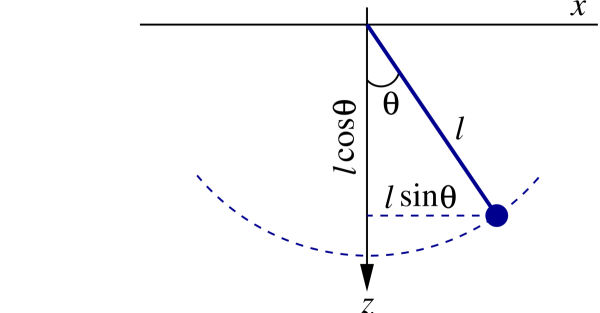
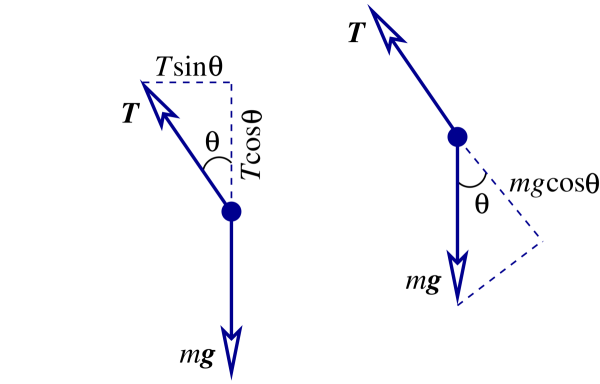
As shown in Fig.1.5, there are two forces acting on the pendulum. The first is gravity, pulling down, and the second is the tension within the rod, which always pulls in the rod's direction. The geometry of the problem suggests that it might be a good idea to involve the polar coordinates introduced in Sec.1.2. Adapting the notation somewhat, we express the Cartesian coordinates $x$ and $z$ of the mass $m$ in terms of the new coordinates $r$ and $\theta$; the relationship is

$$\begin{equation} x = r \sin\theta, \qquad z = r \cos\theta. \tag{1.3.22} \end{equation}$$

At a later stage of the calculation we will incorporate the fact that the distance $r$ between $m$ and the origin of the coordinate system is constant: $r = \ell$. For the moment, however, we shall pretend that $r$ is free to change with time.

The polar coordinates $(r,\theta)$ come with the basis of unit vectors $\boldsymbol{\hat{r}}$ and $\boldsymbol{\hat{\theta}}$, with

$$\boldsymbol{\hat{r}} = \frac{\partial \boldsymbol{r}}{\partial r} = \sin\theta\, \boldsymbol{\hat{x}} + \cos\theta\, \boldsymbol{\hat{z}}$$

and

$$\boldsymbol{\hat{\theta}} = \frac{1}{r} \frac{\partial \boldsymbol{r}}{\partial \theta} = \cos\theta\, \boldsymbol{\hat{x}} - \sin\theta\, \boldsymbol{\hat{z}},$$

where $\boldsymbol{r}(r,\theta) = r\sin\theta\, \boldsymbol{\hat{x}} + r\cos\theta\, \boldsymbol{\hat{z}}$ is the position vector expressed in terms of the polar coordinates. The unit vector $\boldsymbol{\hat{r}}$ points in the direction of increasing $r$ (always away from the origin), while the unit vector $\boldsymbol{\hat{\theta}}$ points in the direction of increasing $\theta$.

As we have seen in Sec.1.2, the acceleration vector of the mass $m$ can be expressed in the polar coordinates and resolved in the new basis vectors. Repeating the calculations carried out there, we find

$$\begin{equation} \boldsymbol{a} = (\ddot{r} - r \dot{\theta}^2)\, \boldsymbol{\hat{r}} + \frac{1}{r} \frac{d}{dt} (r^2 \dot{\theta})\, \boldsymbol{\hat{\theta}}. \tag{1.3.23} \end{equation}$$

The net force acting on the mass $m$ is $\boldsymbol{F} = \boldsymbol{T} + m\boldsymbol{g}$, the vectorial sum of the tension and gravitational forces, respectively. Because the tension is directed along the rod, we have $\boldsymbol{T} = -T \boldsymbol{\hat{r}}$, with $T$ denoting the magnitude of the tension. The force of gravity, on the other hand, is directed along the $z$ direction, and we have $m\boldsymbol{g} = mg \boldsymbol{\hat{z}}$. Resolving this in the new basis (Fig.~1.5), we have $m\boldsymbol{g} = mg\cos\theta\, \boldsymbol{\hat{r}} - mg\sin\theta\, \boldsymbol{\hat{\theta}}$, and the net force is

$$\begin{equation} \boldsymbol{F} = (-T + mg\cos\theta)\, \boldsymbol{\hat{r}} - mg\sin\theta\, \boldsymbol{\hat{\theta}}. \tag{1.3.24} \end{equation}$$

Equating this to $m\boldsymbol{a}$ produces

$$m(\ddot{r} - r \dot{\theta}^2) = -T + mg\cos\theta, \qquad \frac{1}{r} \frac{d}{dt} (r^2 \dot{\theta}) = - g\sin\theta,$$

the equations of motion for the pendulum.

These equations simplify considerably when we finally incorporate the fact that $r = \ell$ and does not change with time (so that $\dot{r} = \ddot{r} = 0$). The first equation gives us an expression for the tension: $T = m(\ell\dot{\theta}^2 + g\cos\theta)$. The second equation reduces to $\ell \ddot{\theta} = -g\sin\theta$, or

$$\begin{equation} \ddot{\theta} + \omega^2 \sin\theta = 0, \tag{1.3.25} \end{equation}$$

where

$$\begin{equation} \omega = \sqrt{g/\ell} \tag{1.3.26} \end{equation}$$

has the dimensions of inverse time (or frequency).

---

Exercise 1.8: Make sure that you can reproduce all the algebra that goes into the derivation of Eqs.(1.3.25) and (1.3.26).

---

---

Exercise 1.9: Equation (1.3.25) can also be derived on the basis of Eq.(1.3.4), $d\boldsymbol{L}/dt = \boldsymbol{N}$, where $\boldsymbol{L} = m \boldsymbol{r} \times \boldsymbol{v}$ is the pendulum's angular momentum and $\boldsymbol{N} = \boldsymbol{r} \times \boldsymbol{F}$ the net torque acting on it. Work through the details and verify that this equation does indeed lead to Eq.(1.3.25). This method of derivation does not require the new basis of unit vectors; all calculations can be carried out in the Cartesian basis.

---

The second-order differential equation of Eq.(1.3.25) determines the motion of the pendulum. It can immediately be integrated once with respect to time. The trick is to multiply Eq.(1.3.25) by $\dot{\theta}$; this gives

$$\ddot{\theta} \dot{\theta} + (\omega^2 \sin\theta) \dot{\theta} = 0.$$

Now note that

$$\ddot{\theta} \dot{\theta} = \frac{1}{2} \frac{d}{dt} \dot{\theta}^2$$

and

$$(\sin\theta) \dot{\theta} = -\frac{d}{dt} \cos\theta.$$

We therefore have

$$\frac{d}{dt} \biggl( \frac{1}{2} \dot{\theta}^2 - \omega^2 \cos\theta \biggr) = 0,$$

or

$$\begin{equation} \frac{1}{2} \dot{\theta}^2 - \omega^2 \cos\theta = \varepsilon = \text{constant}. \tag{1.3.27} \end{equation}$$

This is a first-order differential equation for $\theta(t)$.

It seems intuitively plausible that the conserved quantity $\varepsilon$ should have something to do with the pendulum's total energy $E$. This is indeed the case. The kinetic energy is $T = \frac{1}{2} m (\dot{x}^2 + \dot{z}^2) = \frac{1}{2} m \ell^2 \dot{\theta}^2$, according to our previous results. The potential energy associated with the gravitational force is $V = -mgz = -mg\ell\cos\theta = -m\ell^2\omega^2 \cos\theta$, where we have used Eq.(1.3.26). The potential energy associated with the rod's tension is zero: The tension always acts in the rod's direction, which is always perpendicular to the direction of the motion; the tension does no work on the pendulum. We finally have $E = T+V = m\ell^2 (\frac{1}{2} \dot{\theta}^2 - \omega^2 \cos\theta)$, or

$$\begin{equation} E = m\ell^2 \varepsilon. \tag{1.3.28} \end{equation}$$

We shall call $\varepsilon$ the pendulum's reduced energy. Similarly, we shall call $\frac{1}{2} \dot{\theta}^2$ the reduced kinetic energy and $\nu(\theta) \equiv -\omega^2 \cos\theta$ the reduced potential energy.

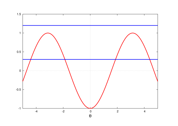
The qualitative features of the pendulum's motion can be understood without further calculation, purely on the basis of the following graphical construction. We draw an energy diagram, a plot of the reduced potential energy $\nu(\theta) = -\omega^2 \cos\theta$ as a function of $\theta$, together with the constant value of the reduced energy $\varepsilon$ (see Fig.1.6). According to Eq.(1.3.27), which we rewrite as

$$\begin{equation} \frac{1}{2} \dot{\theta}^2 = \varepsilon - \nu(\theta), \qquad \nu(\theta) = -\omega^2 \cos\theta, \tag{1.3.29} \end{equation}$$

the difference between $\varepsilon$ and $\nu(\theta)$ is equal to the reduced kinetic energy $\frac{1}{2} \dot{\theta}^2$. For motion to take place this difference must be positive, and a quick examination of the diagram reveals immediately the regions for which $\varepsilon - \nu(\theta) \leq 0$. Motion is possible within these regions, and impossible outside.

For example, when $\varepsilon < \omega^2$ we see that the motion of the pendulum takes place between the two well-defined limits $\theta = \pm\theta_0$; motion is impossible beyond these points. This situation corresponds to ordinary pendulum motion: The weight oscillates back and forth around the vertical axis ($\theta = 0$), with an amplitude $\theta_0$. The diagram reveals that the angular velocity $|\dot{\theta}|$ is maximum when the weight crosses $\theta = 0$, and that the pendulum comes to a momentary rest ($\dot{\theta} = 0$) when $\theta = \pm\theta_0$. This amplitude is determined by setting $\dot{\theta} = 0$ in Eq.(1.3.29); we have

$$\begin{equation} \varepsilon = \nu(\theta_0) = -\omega^2 \cos\theta_0. \tag{1.3.30} \end{equation}$$

This equation can be solved for $\theta_0$ whenever $\varepsilon < \omega^2$; there are no solutions otherwise. When $\varepsilon > \omega^2$ the diagram reveals that there are no intersections between the line $\varepsilon = \text{constant}$ and the curve $\nu(\theta)$. There are no points at which $\frac{1}{2} \dot{\theta}^2 = 0$, $\theta$ is allowed to increase without bound, and the motion is not limited. This high-energy situation corresponds to the weight doing complete revolutions around the pivot point.

Points in the energy diagram at which the line $\varepsilon = \text{constant}$ meets the curve $\nu(\theta)$ are called {\it turning points}. At these points the reduced kinetic energy $\frac{1}{2} \dot{\theta}^2$ drops to zero and $\dot{\theta}$ changes sign, either from the positive to the negative (if $\theta$ was increasing toward $\theta_0$), or from the negative to the positive (if $\theta$ was decreasing toward $-\theta_0$). These are the points at which the pendulum reaches its maximum angle and turns around.

Combining Eqs.(1.3.29) and (1.3.30) gives

$$\begin{equation} \frac{1}{2} \dot{\theta}^2 = \omega^2 (\cos\theta - \cos\theta_0), \tag{1.3.31} \end{equation}$$

and this is a first-order differential equation for $\theta(t)$. This equation, unfortunately, cannot be solved in closed form, unless $\theta_0$ is assumed to be very small (we shall deal separately with this simple case at the end of this subsection). The best we can do is to express $t$ in terms of an integral involving $\theta$. First we take the square root of Eq.(1.3.31),

$$\dot{\theta} = \pm \sqrt{2} \omega \sqrt{\cos\theta - \cos\theta_0},$$

and we solve for $dt$. After integration we get

$$\begin{equation} t = \pm \frac{1}{\sqrt{2}\omega} \int \frac{d\theta}{\sqrt{\cos\theta - \cos\theta_0}} + \text{constant}. \tag{1.3.32} \end{equation}$$

This integral must be evaluated numerically, and the result $t(\theta)$ must be inverted to give $\theta(t)$; the inversion must also be done numerically. To obtain these details requires some labour, and this will not be pursued here. The results of a numerical integration are presented in Fig.1.7.

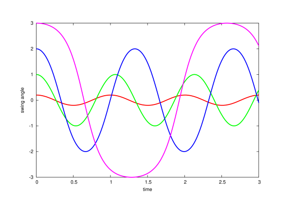
The motion of the pendulum is clearly periodic, and Eq.(1.3.32) allows us to calculate the period $P$, the time required for the pendulum to complete a full cycle of oscillation ($\theta$ going from $-\theta_0$ to $+\theta_0$ and then back to $-\theta_0$.) This is twice the time required to go from $-\theta_0$ to $+\theta_0$, or four times the time required to go from $\theta = 0$ to $\theta = \theta_0$. So the period is given by

$$P = \frac{4}{\sqrt{2}\omega} \int_0^{\theta_0} \frac{d\theta}{\sqrt{\cos\theta - \cos\theta_0}}.$$

To put this integral in standard form we change the variable of integration to

$$z = \frac{\sin {\textstyle \frac{1}{2}} \theta} {\sin {\textstyle \frac{1}{2}} \theta_0}$$

and introduce the parameter

$$\begin{equation} s = \sin {\textstyle \frac{1}{2}} \theta_0. \tag{1.3.33} \end{equation}$$

Simple manipulations reveal that

$$\frac{dz}{d\theta} = \frac{\sqrt{1-s^2 z^2}}{2s}, \qquad \sqrt{\cos\theta - \cos\theta_0} = \sqrt{2} s \sqrt{1-z^2},$$

and the expression for $P$ becomes

$$\begin{equation} P = \frac{4}{\omega} K(s^2), \tag{1.3.34} \end{equation}$$

where

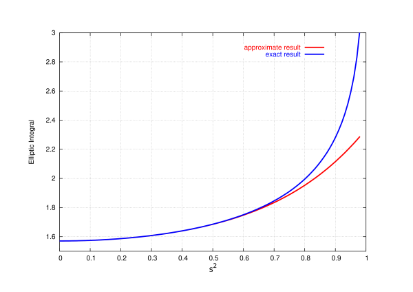
$$\begin{equation} K(s^2) = \int_0^1 \frac{dz}{\sqrt{(1-z^2)(1-s^2 z^2)}} \tag{1.3.35} \end{equation}$$

is a special function known as the complete elliptic integral of the first kind. A plot of this function is shown in Fig.1.8. While this result is perhaps not too revealing, it allows us to conclude that the period increases with the amplitude of the motion. This follows because $P$ depends on $s^2 = \sin^2{\textstyle \frac{1}{2}}\theta_0$ through the elliptic integral.

---

Exercise 1.10: Make sure that you can reproduce all the algebra that goes into the derivation of Eqs.(1.3.34) and (1.3.35)

---

We can be more explicit when $s = \sin{\textstyle \frac{1}{2}} \theta_0$ is fairly small compared with 1. In this situation it is known that the elliptic integral can be approximated by

$$K = \frac{\pi}{2} \biggl[ 1 + \biggl(\frac{1}{2}\biggr)^2 s^2 + \biggl(\frac{1 \cdot 3}{2 \cdot 4}\biggr)^2 s^4 + \biggl(\frac{1 \cdot 3 \cdot 5}{2 \cdot 4 \cdot 6}\biggr)^2 s^6 + \cdots \biggr].$$

Substituting this into Eq.(1.3.34) gives

$$\begin{equation} P = \frac{2\pi}{\omega} \biggl[ 1 + \frac{1}{4} s^2 + \frac{9}{64} s^4 + \frac{25}{256} s^6 + \cdots \biggr]. \tag{1.3.36} \end{equation}$$

When the oscillations are very small, that is when $\theta_0 \ll 1$, we have that $s^2 \ll 1$ and the period is well approximated by the leading term in the power expansion, $P \simeq 2\pi/\omega$. In this limit the period becomes independent of the motion's amplitude.

---

Exercise 1.11: It is not too difficult to derive the preceding approximation to the elliptic integral. When $s^2$ is small the factor $(1-s^2 z^2)^{-1/2}$ inside the integral of Eq.(1.3.35) can be expressed as a Taylor series about $s=0$. Show that this gives $$(1-s^2 z^2)^{-1/2} = 1 + \frac{1}{2} s^2 z^2 + \frac{3}{8} s^4 z^4 + \frac{5}{16} s^6 z^6 + \cdots.$$ With this expansion the elliptic integral becomes $$K = \int_0^1 \frac{dz}{\sqrt{1-z^2}} + \frac{1}{2} s^2 \int_0^1 \frac{z^2\, dz}{\sqrt{1-z^2}} + \frac{3}{8} s^4 \int_0^1 \frac{z^4\, dz}{\sqrt{1-z^2}} + \frac{5}{16} s^6 \int_0^1 \frac{z^6\, dz}{\sqrt{1-z^2}} + \cdots.$$ Evaluate these integrals and verify that your result agrees with the expression quoted in the text.

---

The case of small oscillations is particularly simple to deal with. Go back to Eq.(1.3.25), $\ddot{\theta} + \omega^2 \sin\theta = 0$, and assume that $\theta$ is so small that $\sin\theta$ is well approximated by $\theta$. The equation simplifies to

$$\begin{equation} \ddot{\theta} + \omega^2 \theta = 0, \tag{1.3.37} \end{equation}$$

and we have simple harmonic motion. The general solution to this equation is

$$\begin{equation} \theta(t) = \theta_0 \cos(\omega t + \delta), \tag{1.3.38} \end{equation}$$

where $\theta_0$ is the amplitude and $\delta$ the initial phase. The solution reveals that the period of the motion is $P = 2\pi/\omega$, in complete agreement with our previous results.

1.4 Mechanics of a System of Bodies

1.4.1 Equations of Motion

Generalizing the discussion of the preceding section, we now consider a system of $N$ bodies subjected to their mutual forces. For simplicity we assume that there are no external forces acting on the particles; these would originate from outside the system. Each particle in the system is labeled by a number $A = 1, 2, 3, \cdots, N$. The motion of body $A$ is governed by the equation

$$\begin{equation} m_A \boldsymbol{a}_A = \boldsymbol{F}_A, \tag{1.4.1} \end{equation}$$

where $m_A$ is the mass of the body, $\boldsymbol{a}_A$ its acceleration, and $\boldsymbol{F}_A$ is the force acting on the body due to all other bodies. Relative to an arbitrary choice of origin $O$, the position vector of body $A$ is $\boldsymbol{r}_A(t)$, its velocity is $\boldsymbol{v}_A(t) = \boldsymbol{\dot{r}}_A$, and its acceleration is $\boldsymbol{a}_A(t) = \boldsymbol{\dot{v}}_A = \boldsymbol{\ddot{r}}_A$.

The force acting on body $A$ can be expressed as a sum of individual forces exerted by each other body. We write

$$\begin{equation} \boldsymbol{F}_A = \sum_{B\neq A} \boldsymbol{F}_{AB}. \tag{1.4.2} \end{equation}$$

Here, $\boldsymbol{F}_{AB}$ is the force exerted on $A$ by $B$; the sum over $B$ obviously excludes $A$ because a body does not exert a force on itself. We assume Newton's third law, which states that

$$\begin{equation} \boldsymbol{F}_{BA} = -\boldsymbol{F}_{AB}. \tag{1.4.3} \end{equation}$$

In words, the force exerted on $B$ by $A$ is equal in magnitude and opposite in direction to the force exerted on $A$ by $B$. Suppose, for example, that the force exerted on $A$ by $B$ is repulsive; then the force exerted on $B$ by $A$ will also be repulsive, and it will point in the opposite direction.

1.4.2 Centre of Mass

The centre of mass of a system of $N$ bodies is at a position $\boldsymbol{R}$ which is defined by

$$\begin{equation} \boldsymbol{R} = \frac{1}{M} \sum_A m_A \boldsymbol{r}_A, \tag{1.4.4} \end{equation}$$

where

$$\begin{equation} M = \sum_A m_A \tag{1.4.5} \end{equation}$$

is the total mass of the system.

The centre of mass moves in accordance with Newton's law, which implies

$$\begin{align} M \boldsymbol{\ddot{R}} &= \sum_A m_A \boldsymbol{a}_A \\ &=& \sum_A \boldsymbol{F}_A \\ &= \sum_{A,B,A\neq B} \boldsymbol{F}_{AB}, \end{align}$$

where we have used Eq.(1.4.2). In the last line we sum over both $A$ and $B$ (both from 1 to $N$), but we make sure to exclude all terms for which $A = B$. Let us examine the double sum in the special case of three particles. We have

$$\begin{align} \sum_{A,B,A\neq B} \boldsymbol{F}_{AB} &= \sum_{A=1}^N \sum_{B=1}^N \boldsymbol{F}_{AB} \\ &= \sum_{A=1}^N \bigl( \boldsymbol{F}_{A1} + \boldsymbol{F}_{A2} + \boldsymbol{F}_{A3} \bigr) \\ &= \bigl( \boldsymbol{F}_{21} + \boldsymbol{F}_{31} \bigr) + \bigl( \boldsymbol{F}_{12} + \boldsymbol{F}_{32} \bigr) + \bigl( \boldsymbol{F}_{13} + \boldsymbol{F}_{23} \bigr) \\ &= \bigl( \boldsymbol{F}_{21} + \boldsymbol{F}_{12} \bigr) + \bigl( \boldsymbol{F}_{31} + \boldsymbol{F}_{13} \bigr) + \bigl( \boldsymbol{F}_{32} + \boldsymbol{F}_{23} \bigr) \\ &= \boldsymbol{0}. \end{align}$$

The double sum vanishes by virtue of Newton's third law, and this property remains true for arbitrary values of $N$. We therefore have

$$\begin{equation} \boldsymbol{\ddot{R}} = \boldsymbol{0}, \qquad \Rightarrow \qquad \boldsymbol{R}(t) = \boldsymbol{R}(0) + \boldsymbol{\dot{R}}(0) t. \tag{1.4.6} \end{equation}$$

The centre of mass moves with a uniform velocity, and it therefore defines the origin of another inertial frame.

It is usually convenient to shift the origin of the reference frame to the centre of mass, by defining new positions vectors $\boldsymbol {r'}_A(t)$ according to

$$\begin{equation} \boldsymbol{r'}_A = \boldsymbol{r}_A - \boldsymbol{R}. \tag{1.4.7} \end{equation}$$

It should be kept in mind that the centre of mass defines the origin of an inertial frame only when there are no external forces acting on the particles. When external forces are present each particle moves according to $m_A \boldsymbol{a}_A = \boldsymbol{F}_A^{\rm internal} + \boldsymbol{F}_A^{\rm external}$, where the first term represents the internally-produced force acting on $A$, and the second term represents the external force. It is then easy to show that the centre of mass will move according to $M \boldsymbol{\ddot{R}} = \sum_{A} \boldsymbol{F}_A^{\rm external}$; it is accelerated by the net sum of all the external forces.

---

Exercise 1.12: Prove the preceding statement.

---

1.4.3 Total Linear and Angular Momentum

The total linear momentum of the system of $N$ bodies is defined by

$$\begin{equation} \boldsymbol{P} = \sum_{A} \boldsymbol{p}_A = \sum_{A} m_A \boldsymbol{v}_A, \tag{1.4.8} \end{equation}$$

where $\boldsymbol{p}_A$ are the individual momenta. We have

$$\boldsymbol{P} = \frac{d}{dt} \sum_A m_A \boldsymbol{r}_A,$$

or, according to Eq.(1.4.4),

$$\begin{equation} \boldsymbol{P} = M \boldsymbol{\dot{R}}. \tag{1.4.9} \end{equation}$$

The total momentum therefore follows the motion of the centre of mass. Because $\boldsymbol{\dot{R}}(t) = \boldsymbol{\dot{R}}(0)$ according to Eq.(1.4.6), we have the important statement that {\it the total linear momentum is a constant vector}. If the origin of the inertial frame is at the centre of mass, then $\boldsymbol{R} = \boldsymbol{0}$ and $\boldsymbol{\dot{R}} = \boldsymbol{0}$; this means that $\boldsymbol{P} = \boldsymbol{0}$. In this centre-of-mass frame, the total momentum of the system of particles is zero.

The total angular momentum of the system is

$$\begin{equation} \boldsymbol{L} = \sum_A \boldsymbol{r}_A \times \boldsymbol{p}_A = \sum_A m_A \boldsymbol{r}_A \times \boldsymbol{v}_A. \tag{1.4.10} \end{equation}$$

Its rate of change is calculated as

$$\begin{align} \boldsymbol{\dot{L}} &= \sum_A m_A \bigl( \boldsymbol{v}_A \times \boldsymbol{v}_A + \boldsymbol{r}_A \times \boldsymbol{a}_A \bigr) \\ &= \sum_A \boldsymbol{r}_A \times \boldsymbol{F}_A \\ &= \sum_{A,B,A\neq B} \boldsymbol{r}_A \times \boldsymbol{F}_{AB}, \end{align}$$

where we have again involved Eq.(1.4.2). Let us examine the double sum for the special case of three particles. We have

$$\begin{align} \sum_{A,B,A\neq B} \boldsymbol{r}_A \times \boldsymbol{F}_{AB} &= \sum_A \bigl( \boldsymbol{r}_A \times \boldsymbol{F}_{A1} + \boldsymbol{r}_A \times \boldsymbol{F}_{A2} + \boldsymbol{r}_A \times \boldsymbol{F}_{A3} \bigr) \\ &= \bigl( \boldsymbol{r}_2 \times \boldsymbol{F}_{21} + \boldsymbol{r}_3 \times \boldsymbol{F}_{31} \bigr) + \bigl( \boldsymbol{r}_1 \times \boldsymbol{F}_{12} + \boldsymbol{r}_3 \times \boldsymbol{F}_{32} \bigr) \bigl( \boldsymbol{r}_1 \times \boldsymbol{F}_{13} + \boldsymbol{r}_2 \times \boldsymbol{F}_{23} \bigr) \\ &= \bigl( \boldsymbol{r}_1 - \boldsymbol{r}_2 \bigr) \times \boldsymbol{F}_{12} + \bigl( \boldsymbol{r}_1 - \boldsymbol{r}_3 \bigr) \times \boldsymbol{F}_{13} + \bigl( \boldsymbol{r}_2 - \boldsymbol{r}_3 \bigr) \times \boldsymbol{F}_{23}, \end{align}$$

where we have used Eq.(1.4.3). The vector $\boldsymbol{r}_1 - \boldsymbol{r}_2$ is directed from body 2 to body 1. In most circumstances the force $\boldsymbol{F}_{12}$ also is directed from body 2 to body 1 (or in the opposite direction). Under these conditions the vector product $(\boldsymbol{r}_1 - \boldsymbol{r}_2) \times \boldsymbol{F}_{12}$ is zero, and this is true for all other pairs of bodies. The double sum is therefore zero. These considerations generalize to an arbitrary number of bodies, and we conclude that

$$\begin{equation} \boldsymbol{\dot{L}} = \boldsymbol{0} \tag{1.4.11} \end{equation}$$

whenever the force $\boldsymbol{F}_{AB}$ points in the direction of the relative separation $\boldsymbol{r}_A - \boldsymbol{r}_B$. Under these conditions we have conservation of the system's total angular momentum.

---

Exercise 1.13: Calculate $d \boldsymbol{P}/dt$ and $d \boldsymbol{L}/dt$ when there are also external forces acting on the particles.

---

Let us express the position vector of body $A$ as in Eq.(1.4.7),

$$\begin{equation} \boldsymbol{r}_A = \boldsymbol{R} + \boldsymbol{r'}_A, \tag{1.4.12} \end{equation}$$

where $\boldsymbol{r'}_A$ is its position relative to the centre of mass. We write, similarly,

$$\begin{equation} \boldsymbol{v}_A = \boldsymbol{\dot{R}} + \boldsymbol{v'}_A. \tag{1.4.13} \end{equation}$$

We make these substitutions into Eq.(1.4.10), and get

$$\begin{align} \boldsymbol{L} &= \sum_A m_A \bigl( \boldsymbol{R} + \boldsymbol{r'}_A \bigr) \times \bigl( \boldsymbol{\dot{R}} + \boldsymbol{v'}_A \bigr) \\ &= \sum_A m_A \bigl( \boldsymbol{R} \times \boldsymbol{\dot{R}} + \boldsymbol{R} \times \boldsymbol{v'}_A + \boldsymbol{r'}_A \times \boldsymbol{\dot{R}} + \boldsymbol{r'}_A \times \boldsymbol{v'}_A \bigr) \\ &= \bigl(\boldsymbol{R} \times \boldsymbol{\dot{R}}\bigr) \sum_A m_A + \boldsymbol{R} \times \sum_A m_A \boldsymbol{v'}_A - \boldsymbol{\dot{R}} \times \sum_A m_A \boldsymbol{r'}_A + \sum_A m_A \boldsymbol{r'}_A \times \boldsymbol{v'}_A. \end{align}$$

This mess simplifies. For the first term on the right-hand side we have $\sum_A m_A = M$, the total mass of the system. In the second term we recognize that $\sum_A m_A \boldsymbol{v'}_A$ is the system's total momentum as measured in the centre-of-mass frame; this is zero. The third term vanishes also, and we finally have

$$\begin{equation} \boldsymbol{L} = M \boldsymbol{R} \times \boldsymbol{\dot{R}} + \sum_A m_A \boldsymbol{r'}_A \times \boldsymbol{v'}_A. \tag{1.4.14} \end{equation}$$

In this expression, the first term represents the angular momentum of the centre of mass, while the second term is the total angular momentum of the system of particles relative to the centre of mass. When the origin of the inertial frame is placed at the centre of mass, we have $\boldsymbol{R} = \boldsymbol{0}$ and the first term disappears. In general, we see that $\boldsymbol{L}$ depends on the choice of origin.

1.4.4 Conservation of Energy

The presentation here parallels closely our discussion of Sec.1.3.4 on energy conservation for a single particle. The notation of this section, however, will be slightly more cumbersome, because we now have to keep track of many particles.

We begin by calculating the total work done on all the particles as they move from a configuration labeled 1 to another configuration labeled 2. (This means that in the interval of time over which we follow the particles, each moves from a point 1 to a point 2 on its trajectory.) This is

$$\begin{equation} W_{12} = \sum_A \int_1^2 \boldsymbol{F}_A \cdot d\boldsymbol{r}_A = \sum_A \int_1^2 \boldsymbol{F}_A \cdot \boldsymbol{v}_A\, dt, \tag{1.4.15} \end{equation}$$

where $d\boldsymbol{r}_A = \boldsymbol{v}_A\, dt$ is the displacement vector on the trajectory of particle $A$. Substituting the equations of motion (1.4.1) gives

$$W_{12} = \sum_A \int_1^2 m_A \frac{d \boldsymbol{v}_A}{dt} \cdot \boldsymbol{v}_A\, dt.$$

But since $\boldsymbol{v}_A \cdot d\boldsymbol{v}_A/dt = \frac{1}{2} d v_A^2/dt$, where $v_A^2 = \boldsymbol{v}_A \cdot \boldsymbol{v}_A$, this becomes

$$W_{12} = \sum_A \int_1^2 \frac{d}{dt} \biggl( \frac{1}{2} m_A v_A^2 \biggr)\, dt = \sum_A \bigl[ T_A(2) - T_A(1) \bigr]$$

where $T_A = \frac{1}{2} m_A v_A^2$ is the kinetic energy of particle $A$. Introducing the total kinetic energyof the system

$$\begin{equation} T = \sum_A T_A = \sum_A \frac{1}{2} m_A v_A^2, \tag{1.4.16} \end{equation}$$

we have obtained the statement of the work-energy theorem,

$$\begin{equation} W_{12} = T(2) - T(1). \tag{1.4.17} \end{equation}$$

In words, this states that the total work done on all the particles is equal to the difference in total kinetic energy between the configurations 2 and 1.

---

Exercise 1.14: Express the total kinetic energy of the system in terms of the centre-of-mass quantities $\boldsymbol{R}$, $\boldsymbol{\dot{R}}$ and the relative quantities $\boldsymbol{r'}_A$, $\boldsymbol{v'}_A$. You should find an expression analogous to Eq.(1.4.14).

---

To proceed further we shall assume that the mutual force $\boldsymbol{F}_{AB}$ can be derived from a potential $V_{AB} = V_{BA}$ that depends only on the distance $r_{AB}$ between the bodies $A$ and $B$. We shall therefore have

$$\begin{equation} V_{AB} = V_{AB}(r_{AB}), \qquad r_{AB} \equiv | \boldsymbol{r}_{AB} |, \qquad \boldsymbol{r}_{AB} \equiv \boldsymbol{r}_A - \boldsymbol{r}_B. \tag{1.4.18} \end{equation}$$

The force acting on $A$ exerted by $B$ is given by

$$\begin{equation} \boldsymbol{F}_{AB} = -\boldsymbol{\nabla}_A V_{AB}, \tag{1.4.19} \end{equation}$$

where $\boldsymbol{\nabla}_A = (\partial/\partial x_A, \partial/\partial y_A, \partial/\partial z_A)$ is the gradient operator with respect to the coordinates $\boldsymbol{r}_A = (x_A,y_A,z_A)$ of body $A$. Similarly, the force acting on $B$ exerted by $A$ is

$$\begin{equation} \boldsymbol{F}_{BA} = -\boldsymbol{\nabla}_B V_{AB}, \tag{1.4.20} \end{equation}$$

where $\boldsymbol{\nabla}_B$ us the gradient operator with respect to the coordinates $\boldsymbol{r}_B = (x_B,y_B,z_B)$ of body $B$. (To be fully symmetrical we might have written $\boldsymbol{F}_{BA} = -\boldsymbol{\nabla}_B V_{BA}$, but this produces the same result because $V_{BA}$ is by definition equal to $V_{AB}$.)

Let us verify that $\boldsymbol{F}_{BA} = -\boldsymbol{F}_{AB}$ and that the forces are directed along the vector $\boldsymbol{r}_A - \boldsymbol{r}_B$, that is, in the direction of the relative separation between the two bodies. Let us examine, say, the $x$ component of $\boldsymbol{F}_{AB}$. According to Eq.(1.4.19) we have

$$F_{AB, x} = -\frac{\partial}{\partial x_A} V_{AB}.$$

Because $V_{AB}$ depends on $x_A$ only through its dependence on the distance $r_{AB}$, we apply the chain rule to evaluate the partial derivative:

$$F_{AB,x} = -\frac{d V_{AB}}{d r_{AB}} \frac{\partial r_{AB}}{\partial x_A} = - V_{AB}' \frac{\partial r_{AB}}{\partial x_A},$$

where the prime indicates differentiation with respect to $r_{AB}$. To calculate the partial derivative of $r_{AB}$ with respect to $x_A$ we start with the definition

$$r^2_{AB} = \bigl(x_A - x_B\bigr)^2 + \bigl(y_A - y_B\bigr)^2 + \bigl(z_A - z_B\bigr)^2.$$

Differentiating both sides gives

$$2 r_{AB} \frac{\partial r_{AB}}{\partial x_A} = 2 \bigl( x_A - x_B \bigr),$$

and finally,

$$\frac{\partial r_{AB}}{\partial x_A} = \frac{x_A - x_B}{r_{AB}}.$$

Returning to our main calculation we find that the $x$ component of the force is

$$F_{AB,x} = -\frac{x_A - x_B}{r_{AB}} V'_{AB},$$

and very similar calculations would reveal also the $y$ and $z$ components. The complete vectorial expression is

$$\begin{equation} \boldsymbol{F}_{AB} = -\frac{\boldsymbol{r}_{AB}}{r_{AB}} V'_{AB}, \qquad V'_{AB} = \frac{d V_{AB}}{d r_{AB}}. \tag{1.4.21} \end{equation}$$

This shows that $F_{AB}$ is indeed directed along $\boldsymbol{r}_{AB} = \boldsymbol{r}_A - \boldsymbol{r}_B$.

We now calculate $\boldsymbol{F}_{BA}$. Looking also at its $x$ component we get from Eq.(1.4.20) that

$$F_{BA,x} = -\frac{d V_{AB}}{d r_{AB}} \frac{\partial r_{AB}}{\partial x_B} = -V_{AB}' \frac{\partial r_{AB}}{\partial x_B}.$$

Repeating the same steps as before we find that

$$\frac{\partial r_{AB}}{\partial x_B} = -\frac{x_A - x_B}{r_{AB}},$$

which differs by a sign from the preceding expression for $\partial r_{AB}/\partial x_A$. We finally obtain

$$F_{BA,x} = \frac{x_A - x_B}{r_{AB}} V'_{AB}$$

and the vectorial generalization

$$\begin{equation} \boldsymbol{F}_{BA} = \frac{\boldsymbol{r}_{AB}}{r_{AB}} V'_{AB}. \tag{1.4.22} \end{equation}$$

This also is directed along $\boldsymbol{r}_{AB} = \boldsymbol{r}_A - \boldsymbol{r}_B$. Comparing Eqs.(1.4.21) and (1.4.22) shows that, as required, $\boldsymbol{F}_{BA} = -\boldsymbol{F}_{AB}$.

The calculations presented above are important and they occur frequently. To go through them with some efficiency it is useful to memorize the rule $\boldsymbol{\nabla}_B V_{AB} = - \boldsymbol{\nabla}_A V_{AB}$, which is valid whenever $V_{AB}$ depends on $\boldsymbol{r}_A$ and $\boldsymbol{r}_B$ only through its dependence on $r_{AB} = |\boldsymbol{r}_A - \boldsymbol{r}_B|$.

Having made our assumptions regarding the mutual forces $\boldsymbol{F}_{AB}$, we now return to the work integral of Eq.(1.4.15). Substituting Eq.(1.4.2) gives

$$W_{12} = \sum_{A,B,A\neq B} \int_1^2 \boldsymbol{F}_{AB} \cdot d\boldsymbol{r}_A.$$

To examine this we again specialize to the case of three particles. We have

$$\begin{align} W_{12} &= \int_1^2 \bigl( \boldsymbol{F}_{21} \cdot d\boldsymbol{r}_2 + \boldsymbol{F}_{31} \cdot d\boldsymbol{r}_3 + \boldsymbol{F}_{12} \cdot d\boldsymbol{r}_1 + \boldsymbol{F}_{32} \cdot d\boldsymbol{r}_3 + \boldsymbol{F}_{13} \cdot d\boldsymbol{r}_1 + \boldsymbol{F}_{23} \cdot d\boldsymbol{r}_2 \bigr) \\ &= \int_1^2 \Bigl[ \boldsymbol{F}_{12} \cdot \bigl( d\boldsymbol{r}_1 - d\boldsymbol{r}_2 \bigr) + \boldsymbol{F}_{13} \cdot \bigl( d\boldsymbol{r}_1 - d\boldsymbol{r}_3 \bigr) + \boldsymbol{F}_{23} \cdot \bigl( d\boldsymbol{r}_2 - d\boldsymbol{r}_3 \bigr) \Bigr]. \end{align}$$

But $d\boldsymbol{r}_1 - d\boldsymbol{r}_2 = d(\boldsymbol{r}_1 - \boldsymbol{r}_2) = d\boldsymbol{r}_{12}$, so this can be expressed as

$$W_{12} = \int_1^2 \bigl( \boldsymbol{F}_{12} \cdot d\boldsymbol{r}_{12} + \boldsymbol{F}_{13} \cdot d\boldsymbol{r}_{13} + \boldsymbol{F}_{23} \cdot d\boldsymbol{r}_{23} \bigr).$$

At this stage of the derivation we incorporate the fact that the mutual forces are derived from a potential. As we have seen, $\boldsymbol{F}_{12} = -\boldsymbol{\nabla}_1 V_{12}$, where $\boldsymbol{\nabla}_1 = (\partial/\partial x_1, \partial/\partial y_1, \partial/\partial z_1)$. But since $V_{12}$ depends on $(x_1,y_1,z_1)$ only through its dependence on $(x_{12},y_{12},z_{12})$ (where, for example, $x_{12} = x_1 - x_2$), the force can also be expressed as $\boldsymbol{F}_{12} = -\boldsymbol{\nabla}_{12} V_{12}$, where $\boldsymbol{\nabla}_{12}$ is the gradient operator with respect to $\boldsymbol{r}_{12} = (x_{12},y_{12},z_{12})$,

$$\boldsymbol{\nabla}_{12} = \biggl( \frac{\partial}{\partial x_{12}}, \frac{\partial}{\partial y_{12}}, \frac{\partial}{\partial z_{12}} \biggr).$$

This is possible because $\partial x_{12}/\partial x_1 = 1$, and so on.

So we now have

$$W_{12} = \int_1^2 \bigl( -\boldsymbol{\nabla}_{12} V_{12} \cdot d\boldsymbol{r}_{12} - \boldsymbol{\nabla}_{13} V_{13} \cdot d\boldsymbol{r}_{13} - \boldsymbol{\nabla}_{23} V_{23} \cdot d\boldsymbol{r}_{23} \bigr).$$

Each integral can be evaluated (refer back to Sec.1.3.1), giving

$$\begin{align} W_{12} &= -\bigl[ V_{12}(2) - V_{12}(1) \/bigr] - \bigl[ V_{13}(2) - V_{13}(1) \bigr] - \bigl[ V_{23}(2) - V_{23}(1) \bigr] \equiv& -\bigl[ V_{12} + V_{13} + V_{23} \bigr]^2_1. \end{align}$$

Since $V_{21} = V_{12}$ and so on, we may write this as

$$W_{12} = -\frac{1}{2} \bigl[ V_{12} + V_{13} + V_{21} + V_{23} + V_{31} + V_{32} \bigr]^2_1,$$

where we now sum over all possible pairs of indices, provided that each index is not repeated. Generalizing to an arbitrary number of particles, this is

$$W_{12} = -\biggl[ \frac{1}{2} \sum_{A,B,A \neq B} V_{AB} \biggr]^2_1.$$

We define the total potential energy of the system to be

$$\begin{equation} V = \frac{1}{2} \sum_{A,B,A \neq B} V_{AB}. \tag{1.4.23} \end{equation}$$

We have finally established that the total mechanical energy of the system,

$$\begin{equation} E = T + V = \sum_A \frac{1}{2} m_A v_A^2 + \frac{1}{2} \sum_{A,B,A \neq B} V_{AB}(r_{AB}), \tag{1.4.24} \end{equation}$$

stays unchanged as the particles move from configuration 1 to configuration 2. We recall that the mutual potentials $V_{AB}$ are assumed to depend on $r_{AB} = |\boldsymbol{r}_A - \boldsymbol{r}_B|$ only; the mutual forces are then given by Eqs.(1.4.21) and (1.4.22). This is the statement of energy conservation for a system of particles.

---

Exercise 1.15: Starting from the definition of Eq.(1.4.24), prove directly that $dE/dt = 0$.

---

1.5 Kepler's Problem

To give concreteness to the formal developments of the preceding section we examine, in this section, the specific situation of two bodies subjected to their mutual gravitational forces. This could be the Earth-Moon system, or the Sun-Jupiter system, or again a binary system of two main-sequence stars. Our goal is to determine the motion of the two bodies, that is, to find a solution to Kepler's problem.

1.5.1 Gravitational Force

The force acting on body 1 due to the gravity of body 2 has a magnitude $G m_1 m_2 / r^2_{12}$, where $G$ is Newton's gravitational constant, $m_1$ the mass of body 1, $m_2$ the mass of body 2, and $r_{12}$ is the distance between the two bodies. The force is directed along the vector $\boldsymbol{r}_2 - \boldsymbol{r}_1$, which points from body 1 to body 2. Introducing the notation

$$\begin{equation} \boldsymbol{r} = \boldsymbol{r}_1 - \boldsymbol{r}_2, \qquad r = |\boldsymbol{r}_1 - \boldsymbol{r}_2| \equiv r_{12}, \tag{1.5.1} \end{equation}$$

we write

$$\begin{equation} \boldsymbol{F}_{12} = -G m_1 m_2 \frac{\boldsymbol{r}}{r^3}. \tag{1.5.2} \end{equation}$$

The force acting on body 2 due to the gravity of body 1 is

$$\begin{equation} \boldsymbol{F}_{21} = G m_1 m_2 \frac{\boldsymbol{r}}{r^3}, \tag{1.5.3} \end{equation}$$

and it is directed along $\boldsymbol{r}_1 - \boldsymbol{r}_2$, which points from body 2 to body 1.

These forces can be derived from a mutual potential

$$\begin{equation} V_{12} = - \frac{G m_1 m_2}{r}. \label{1.5.4} \end{equation}$$

This means that the force of Eq.(1.5.2) is given by

$$\begin{equation} \boldsymbol{F}_{12} = -\boldsymbol{\nabla}_1 V_{12}, \tag{1.5.5} \end{equation}$$

where $\boldsymbol{\nabla}_1$ is the gradient operator with respect to the coordinates $\boldsymbol{r}_1 = (x_1,y_1,z_1)$ of body 1. Similarly, the force of Eq.(1.5.3) can be expressed as

$$\begin{equation} \boldsymbol{F}_{21} = -\boldsymbol{\nabla}_2 V_{12}, \tag{1.5.6} \end{equation}$$

where $\boldsymbol{\nabla}_2$ is the gradient operator with respect to the coordinates $\boldsymbol{r}_2 = (x_2,y_2,z_2)$ of body 2. To verify these statements, let us calculate, say, the $z$ component of $\boldsymbol{F}_{21}$. We have

$$F_{21,z} = -\frac{\partial V_{12}}{\partial z_2} = -\frac{d V_{12}}{dr} \frac{\partial r}{\partial z_2}.$$

The first factor is

$$\frac{d V_{12}}{dr} = \frac{G m_1 m_2}{r^2},$$

and to calculate the second factor we start with

$$r^2 = (x_1-x_2)^2 + (y_1-y_2)^2 + (z_1-z_2)^2$$

and differentiate both sides with respect to $z_2$. This gives

$$2 r \frac{\partial r}{\partial z_2} = -2 (z_1-z_2)$$

or

$$\frac{\partial r}{\partial z_2} = -\frac{z_1 - z_2}{r}.$$

So finally,

$$F_{21,z} = G m_1 m_2 \frac{z_1-z_2}{r^3},$$

and this is clearly compatible with Eq.(1.5.3). Similar calculations would return all other components of $\boldsymbol{F}_{21}$ and all components of $\boldsymbol{F}_{12}$, and Eqs.(1.5.5) and (1.5.6) would be fully verified.

According to Eq.(1.4.23), the total potential energy of the two-body system is

$$V = \frac{1}{2} \sum_{A,B,A \neq B} V_{AB} = \frac{1}{2} (V_{12} + V_{21}),$$

or

$$\begin{equation} V = V_{12}. \tag{1.5.7} \end{equation}$$

This result will allow us, in the following subsections, to omit the label ``12'' from the mutual potential; we shall write, simply, $V_{12} = V = -G m_1 m_2/r$.

1.5.2 Equations of Motion

Newton's equations for the two bodies are $m_1 \boldsymbol{\ddot{r}}_1 = \boldsymbol{F}_{12} = -G m_1 m_2 \boldsymbol{r}/r^3$ and $m_2 \boldsymbol{\ddot{r}}_2 = \boldsymbol{F}_{21} = G m_1 m_2 \boldsymbol{r}/r^3$. Simplifying, we arrive at

$$\begin{equation} \boldsymbol{\ddot{r}}_1 = -G m_2 \frac{\boldsymbol{r}}{r^3} \tag{1.5.8} \end{equation}$$

and

$$\begin{equation} \boldsymbol{\ddot{r}}_2 = G m_1 \frac{\boldsymbol{r}}{r^3}, \tag{1.5.9} \end{equation}$$

where, we recall, $\boldsymbol{r} = \boldsymbol{r}_1 - \boldsymbol{r}_2$ and $r = |\boldsymbol{r}|$.

The position vectors $\boldsymbol{r}_1$ and $\boldsymbol{r}_2$ can be expressed in terms of $\boldsymbol{R}$, the position of the centre of mass, and $\boldsymbol{r}$, the relative position. We have, according to Eq.(1.4.4), $M \boldsymbol{R} = m_1 \boldsymbol{r}_1 + m_2 \boldsymbol{r}_2$, where $M = m_1 + m_2$ is the total mass. Simple algebra gives

$$\begin{equation} \boldsymbol{r}_1 = \boldsymbol{R} + \frac{m_2}{M} \boldsymbol{r} \tag{1.5.10} \end{equation}$$

and

$$\begin{equation} \boldsymbol{r}_2 = \boldsymbol{R} - \frac{m_1}{M} \boldsymbol{r}. \tag{1.5.11} \end{equation}$$

The motion of the centre of mass is determined by the equation $M \boldsymbol{\ddot{R}} = m_1 \boldsymbol{\ddot{r}}_1 + m_2 \boldsymbol{\ddot{r}}_2 = -G m_1 m_2 \boldsymbol{r}/r^3 + G m_1 m_2 \boldsymbol{r}/r^3 = \boldsymbol{0}$. As we had discovered in Sec.1.4.2, the centre of mass moves uniformly:

$$\begin{equation} \boldsymbol{R}(t) = \boldsymbol{R}(0) + \boldsymbol{\dot{R}}(0) t. \tag{1.5.12} \end{equation}$$

The motion of the relative position, on the other hand, is determined by the equation $\boldsymbol{\ddot{r}} = \boldsymbol{\ddot{r}}_1 - \boldsymbol{\ddot{r}}_2 = -G m_2 \boldsymbol{r}/r^3 - G m_1 \boldsymbol{r}/r^3$, or

$$\begin{equation} \boldsymbol{\ddot{r}} = - G M \frac{\boldsymbol{r}}{r^3}, \qquad M = m_1 + m_2. \tag{1.5.13} \end{equation}$$

---

Exercise 1.16: Verify Eqs.(1.5.10) and (1.5.11).

---

The centre of mass defines the origin of an inertial frame, and the mathematical description of the two-body system is simplest in this reference frame. We shall therefore set $\boldsymbol{R} = \boldsymbol{0}$, which brings Eqs.(1.5.10) and (1.5.11) to the simpler form

$$\begin{equation} \boldsymbol{r}_1 = \frac{m_2}{M} \boldsymbol{r}, \qquad \boldsymbol{r}_2 = - \frac{m_1}{M} \boldsymbol{r}. \tag{1.5.14} \end{equation}$$

The vector $\boldsymbol{r}(t)$ is determined by integrating Eq.(1.5.13). Once the solution is known we obtain immediately, from Eqs.(1.5.14), the vectors $\boldsymbol{r}_1(t)$ and $\boldsymbol{r}_2(t)$, which describe the trajectories of the two individual bodies. In Eq.(1.5.13) we have the reduction of our original two-body problem to a simpler effective one-body problem. The effective body is fictitious; it moves with a position vector $\boldsymbol{r}(t)$ in the gravitational field of another fictitious mass $M = m_1 + m_2$ situated at the centre of mass of the original system.

1.5.3 Conservation of Angular Momemtum

From Eq.(1.5.13) we can immediately derive the statement

$$\boldsymbol{r} \times \boldsymbol{\ddot{r}} = -GM \frac{\boldsymbol{r} \times \boldsymbol{r}}{r^3} = \boldsymbol{0}.$$

But $d(\boldsymbol{r} \times \boldsymbol{\dot{r}})/dt = \boldsymbol{\dot{r}} \times \boldsymbol{\dot{r}} + \boldsymbol{r} \times \boldsymbol{\ddot{r}} = \boldsymbol{r} \times \boldsymbol{\ddot{r}}$, and it follows that $d(\boldsymbol{r} \times \boldsymbol{\dot{r}})/dt = \boldsymbol{0}$. The vector

$$\begin{equation} \boldsymbol{h} = \boldsymbol{r} \times \boldsymbol{\dot{r}} \tag{1.5.15} \end{equation}$$

is therefore constant during the motion. This must be related to the system's total angular momentum which, according to the discussion of Sec.1.4.3, is also a constant vector. The definition of Eq.(1.4.10) gives

$$\boldsymbol{L} = \sum_A m_A \boldsymbol{r}_A \times \boldsymbol{\dot{r}}_A = m_1 \boldsymbol{r}_1 \times \boldsymbol{\dot{r}}_1 + m_2 \boldsymbol{r}_2 \times \boldsymbol{\dot{r}}_2.$$

Substitution of Eqs.(1.5.14) gives

$$\begin{equation} \boldsymbol{L} = \frac{m_1 m_2}{M} \boldsymbol{h}, \tag{1.5.16} \end{equation}$$

and we find that, sure enough, the vector $\boldsymbol{h}$ is a rescaled version of the total angular-momentum vector. We shall call $\boldsymbol{h}$ the reduced angular-momentum vector of our two-body system.

The position vector $\boldsymbol{r}(t)$ must be at all times orthogonal to the constant vector $\boldsymbol{h}$, because $\boldsymbol{r} \cdot \boldsymbol{h} = \boldsymbol{r} \cdot (\boldsymbol{r} \times \boldsymbol{\dot{r}}) = 0$. This simple fact has the far-reaching consequence that the motion must always take place within a plane that is orthogonal to the fixed direction of the vector $\boldsymbol{h}$. The planar nature of the motion is illustrated in Fig.1.9.

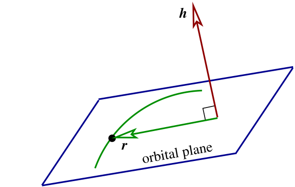
Conservation of total angular momentum therefore implies planar motion. To describe this mathematically we orient the coordinate system so that the orbital plane is the $x$-$y$ plane, and we direct the vector $\boldsymbol{h}$ along the $z$ axis. We have

$$\begin{align} \boldsymbol{r}(t) &= x(t) \boldsymbol{\hat{x}} + y(t) \boldsymbol{\hat{y}}, \tag{1.5.17} \\ \boldsymbol{\dot{r}}(t) &= \dot{x}(t) \boldsymbol{\hat{x}} + \dot{y}(t) \boldsymbol{\hat{y}}, \tag{1.5.18} \end{align}$$

and

$$\begin{equation} \boldsymbol{h} = h \boldsymbol{\hat{z}}. \tag{1.5.19} \end{equation}$$

A simple calculation, based on Eqs.(1.5.15) and (1.5.17)--(1.5.19), reveals that

$$\begin{equation} h = x \dot{y} - y \dot{x} = \text{constant}. \tag{1.5.20} \end{equation}$$

---

Exercise 1.17: Verify Eq.(1.5.20).

---

1.5.4 Polar Coordinates

To proceed with our calculations it is convenient to involve the polar coordinates $r$ and $\phi$ that were first introduced in Sec.1.2. These, we recall, are defined by

$$\begin{equation} x = r \cos\phi, \qquad y = r \sin\phi. \tag{1.5.21} \end{equation}$$

In terms of the new coordinates and the associated basis of unit vectors $\boldsymbol{\hat{r}}$ and $\boldsymbol{\hat{\phi}}$, we have

$$\begin{align} \boldsymbol{r} &= r\, \boldsymbol{\hat{r}}, \tag{1.5.22} \\ \boldsymbol{v} &= \dot{r}\, \boldsymbol{\hat{r}} + r\dot{\phi}\, \boldsymbol{\hat{\phi}}, \tag{1.5.23} \\ \boldsymbol{a} &= \bigl( \ddot{r} - r \dot{\phi}^2 \bigr) \boldsymbol{\hat{r}} + \frac{1}{r} \frac{d}{dt} \bigl( r^2 \dot{\phi} \bigr) \boldsymbol{\hat{\phi}} \tag{1.5.24} \end{align}$$

for the position, velocity, and acceleration vectors, respectively.

If we now substitute Eq.(1.5.24) for $\boldsymbol{a} = \boldsymbol{\ddot{r}}$ into the equations of motion of Eq.(1.5.13), we obtain

$$\bigl( \ddot{r} - r \dot{\phi}^2 \bigr) \boldsymbol{\hat{r}} + \frac{1}{r} \frac{d}{dt} \bigl( r^2 \dot{\phi} \bigr) \boldsymbol{\hat{\phi}} = -\frac{GM}{r^3} \boldsymbol{r} = -\frac{GM}{r^2} \boldsymbol{hat{r}}.$$

Equating the radial components of both sides gives

$$\begin{equation} \ddot{r} - r \dot{\phi}^2 = -\frac{GM}{r^2}, \tag{1.5.25} \end{equation}$$

while equating the angular components gives

$$\begin{equation} \frac{d}{dt} \bigl( r^2 \dot{\phi} \bigr) = 0. \tag{1.5.26} \end{equation}$$

These are the equations of motion of the effective one-body problem, expressed in their simplest form in terms of polar coordinates. In the following subsections we will endeavour to find solutions to these equations.

1.5.5 Kepler's Second Law

Kepler's second law states that the position vector of a planet orbiting the Sun sweeps out equal areas in equal times. The statement generalizes to any two massive bodies, and in this case the position vector refers specifically to the relative separation $\boldsymbol{r}(t)$ between the two bodies. This law comes as an immediate consequence of Eq.(1.5.26), which implies the conservation statement $r^2 \dot{\phi} = \text{constant}$.

Let us first show that this constant is in fact $h$, the magnitude of the constant vector $\boldsymbol{h}$ defined by Eq.(1.5.15). According to Eq.(1.5.20), this is given by $h = x \dot{y} - y \dot{x}$. Making use of Eqs.(1.5.21), we write this as

$$h = (r\cos\phi) (\dot{r} \sin\phi + r \dot{\phi} \cos\phi) - (r\sin\phi) (\dot{r} \cos\phi - r \dot{\phi} \sin\phi).$$

Simplifying this we obtain

$$\begin{equation} h = r^2 \dot{\phi} = \text{constant}, \tag{1.5.27} \end{equation}$$

the expected result.

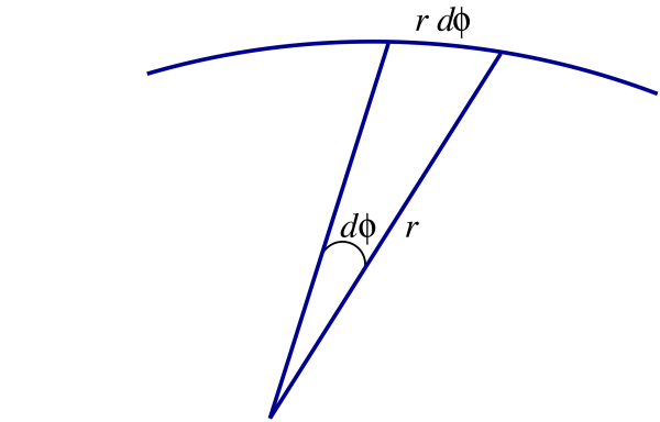
The fact that $r^2 \dot{\phi}$ is conserved gives us our statement of the second law. Consider Fig.1.10. During an interval $dt$ of time the position vector moves by an angle $d\phi$ and sweeps out an area $dA$. To a good approximation the area is shaped as a triangle and we have $dA = \frac{1}{2} r (r\, d\phi) = \frac{1}{2} r^2\, d\phi$. The rate at which the position vector sweeps out this area is therefore

$$\begin{equation} \frac{dA}{dt} = \frac{1}{2} r^2 \dot{\phi} = \frac{1}{2} h. \tag{1.5.28} \end{equation}$$

This is a constant, and we have the mathematical statement of Kepler's second law.

1.5.6 Conservation of Energy

With the substitution $\dot{\phi} = h/r^2$ obtained from Eq.(1.5.25), Eq.(1.5.27) becomes

$$\begin{equation} \ddot{r} + \frac{GM}{r^2} - \frac{h^2}{r^3} = 0. \tag{1.5.29} \end{equation}$$

This equation can immediately be integrated by multiplying all members by $\dot{r}$. (Recall that we used the same trick back in Sec.1.3.7 We have

$$\begin{align} \ddot{r} \dot{r} &= \frac{d}{dt} \biggl( \frac{1}{2} \dot{r}^2 \biggr), \\ \frac{GM}{r^2} \dot{r} &= \frac{d}{dt} \biggl( -\frac{GM}{r} \biggr), \\ -\frac{h^2}{r^3} \dot{r} &= \frac{d}{dt} \biggl( \frac{h^2}{2r^2} \biggr), \end{align}$$

and the preceding equation becomes

$$\frac{d}{dt} \biggl( \frac{1}{2} \dot{r}^2 - \frac{GM}{r} + \frac{h^2}{2r^2} \biggr) = 0.$$

This implies $\frac{1}{2} \dot{r}^2 - GM/r + h^2/(2r^2) = \varepsilon$, where $\varepsilon$ is the constant of integration.

We shall write this result in the form

$$\begin{equation} \frac{1}{2} \dot{r}^2 + \nu(r) = \varepsilon, \tag{1.5.30} \end{equation}$$

with

$$\begin{equation} \nu(r) = -\frac{GM}{r} + \frac{h^2}{2r^2}. \tag{1.5.31} \end{equation}$$

The first term on the left of Eq.(1.5.30) can be thought of as a reduced kinetic energy for the radial component of the motion. The second term is a reduced effective potential for this motion, and the constant $\varepsilon$ is a reduced total energy. (Recall that we introduced this terminology back in Sec.1.3.7; by ``reduced'' we mean a rescaled version of the usual quantities.)

The reduced energy $\varepsilon$ is directly related to the system's true total energy $E$. Let us calculate it. The system's total kinetic energy is $T = \frac{1}{2} m_1 |\boldsymbol{\dot{r}}_1|^2 + \frac{1}{2} m_2 |\boldsymbol{\dot{r}}_2|^2$, and according to Eqs.(1.5.4) and (1.5.7), the potential energy is $V = -G m_1 m_2 /r$. The total energy is therefore

$$E = \frac{1}{2} m_1 |\boldsymbol{\dot{r}}_1|^2 + \frac{1}{2} m_2 |\boldsymbol{\dot{r}}_2|^2 - \frac{G m_1 m_2}{r}.$$

After involving Eq.(1.5.14) and cleaning up the algebra, this becomes

$$\begin{equation} E = \frac{m_1 m_2}{M} \biggl( \frac{1}{2} |\boldsymbol{\dot{r}}|^2 - \frac{GM}{r} \biggr). \tag{1.5.32} \end{equation}$$

Now Eq.(1.5.23) states $\boldsymbol{\dot{r}} = \boldsymbol{v} = \dot{r} \boldsymbol{\hat{r}} + r\dot{\phi} \boldsymbol{\hat{\phi}}$, so that $|\boldsymbol{\dot{r}}|^2 = \dot{r}^2 + r^2 \dot{\phi}^2 = \dot{r}^2 + h^2/r^2$. So

$$E = \frac{m_1 m_2}{M} \biggl( \frac{1}{2} \dot{r}^2 - \frac{GM}{r} + \frac{h^2}{2r^2} \biggr),$$

and comparing this with Eqs.(1.5.30) and (1.5.31) yields

$$\begin{equation} E = \frac{m_1 m_2}{M} \varepsilon. \tag{1.5.33} \end{equation}$$

As promised, $\varepsilon$ is a rescaled version of the total energy $E$. Recall that back in Sec.1.5.3 we had similarly obtained $\boldsymbol{L} = (m_1 m_2/M) \boldsymbol{h}$.

---

Exercise 1.18: Verify Eq.(1.5.32) and check the algebra leading to Eq.(1.5.33).

---

1.5.7 Qualitative Description of the Orbital Momentum

The equations of motion have been reduced to the first-order form of Eqs.(1.5.27) and (1.5.30), with the effective potential $\nu(r)$ given by Eq.(1.5.31). The equation $\dot{\phi} = h/r^2$ informs us that $\phi$ increases monotonically with $t$: If $h$ is positive $\dot{\phi}$ is always greater than zero and $\phi(t)$ is an increasing function; if $h$ is negative $\dot{\phi}$ is always smaller than zero and $\phi(t)$ is then a decreasing function. (The case $h = 0$ will be dealt with separately later.) The equation

$$\frac{1}{2} \dot{r}^2 + \nu(r) = \varepsilon$$

governs the radial component of the motion. As in Sec.1.3.7 we will describe this qualitatively by constructing an energy diagram, a plot of the effective potential $\nu(r)$ together with the constant value of the reduced energy $\varepsilon$. The energy diagram is shown in Fig.1.11. Recall the two main features of such diagrams: (i) The difference between $\varepsilon$ and $\nu(r)$ represents $\frac{1}{2} \dot{r}^2$, the reduced kinetic energy, which must be positive; and (ii) points on the diagram for which $\nu(r) = \varepsilon$ represent turning points of the motion, at which $\dot{r}$ changes sign, either from positive to negative, or from negative to positive.

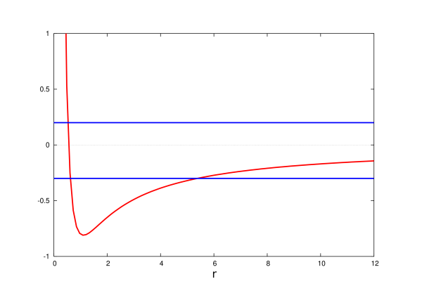
Because the effective potential can be negative, it is possible for $\varepsilon$ to be either negative or positive. The nature of the motion depends sensitively on this sign.

When $\varepsilon < 0$ the motion takes place between two turning points at $r = r_{\rm min}$ and $r = r_{\rm max}$. The motion is bounded, and as we shall see, the orbit possesses an elliptical shape. When $\varepsilon$ is equal to the minimum value of the effective potential, $\varepsilon = \nu_{\rm min} < 0$, motion can take place only at $r=r_0$, the radius at which the minimum occurs, which is defined by $\nu(r_0) = \nu_{\rm min}$. The orbit is then circular, because $\dot{r}$ is always zero and $r$ can therefore never change with time.

When $\varepsilon > 0$ the motion takes place only to the right of a single turning point at $r = r_{\rm min}$. The motion proceeds from $r=\infty$ (where $\nu = 0$ and $\frac{1}{2} \dot{r}^2 = \varepsilon$) down to $r = r_{\rm min}$ (where $\dot{r}$ changes sign from negative to positive), and then back to $r = \infty$. The particle traces a hyperbola in the orbital plane, and the motion is said to be hyperbolic.

When $\varepsilon = 0$ the situation is qualitatively the same as before (for $\varepsilon > 0$). The only difference is that the particle now starts at $r = \infty$ with a zero radial velocity, because $\frac{1}{2} \dot{r}^2 = \varepsilon = 0$. The particle then traces a parabola in the orbital plane, and the motion is parabolic.

1.5.8 Circular Orbits

Circular orbits are especially simple to describe. To have circular motion we need both $\dot{r}$ and $\ddot{r}$ to be zero, so that $r$ always stays constant. The condition $\dot{r} = 0$ is not sufficient, because $\dot{r}$ might just happen to be in the process of changing sign at a turning point; we need a permanent turning point, which we get by also imposing $\ddot{r} = 0$. To get $\dot{r} = 0$ we need to impose

$$\varepsilon = \nu(r_0) = -\frac{GM}{r_0} + \frac{h^2}{2r_0^2},$$

where $r_0$ is the orbital radius. To get $\ddot{r} = 0$ we look back at Eq.(1.5.29) and impose

$$0 = \frac{GM}{r_0^2} - \frac{h^2}{r_0^3} = \nu'(r_0),$$

in which a prime indicates differentiation with respect to $r$. The second equation determines $h$ in terms of $r_0$: we get $h^2 = GMr_0$, or

$$\begin{equation} h = \sqrt{G M r_0}, \tag{1.5.34} \end{equation}$$

if we choose a positive sign for $h$. The first equation determines $\varepsilon$ also in terms of $r_0$: we get $\varepsilon = -GM/r_0 + GM/(2r_0)$, or

$$\begin{equation} \varepsilon = -\frac{GM}{2r_0}. \tag{1.5.35} \end{equation}$$

The angular velocity of a circular orbit is given by $\dot{\phi} = h/r_0^2 = \sqrt{G M r_0}/r_0^2$, or

$$\begin{equation} \dot{\phi} = \sqrt{ \frac{GM}{r_0^3} }. \tag{1.5.36} \end{equation}$$

The orbital period $P$ is the time required for $\phi$ to advance by $2\pi$. We have $\sqrt{GM/r_0^3} = 2\pi/P$, which gives

$$\begin{equation} P = 2\pi \sqrt{ \frac{r_0^3}{GM} }. \tag{1.5.37} \end{equation}$$

This equation states that $P^2 \propto r_0^3$, and we have the statement of Kepler's third law for circular orbits.

1.5.9 Shape of Orbits

To go beyond the qualitative description of the orbit we must now fully integrate the equations of motion. We shall, to begin with, eliminate the time from the equations and focus on the geometrical appearance of the orbit; we shall, in other words, derive a differential equation for $r(\phi)$ and solve it. We will return later with a description of the motion in time.

We go back to Eq.(1.5.29),

$$\ddot{r} + \frac{GM}{r^2} - \frac{h^2}{r^3} = 0,$$

and to Eq.(1.5.27),

$$\dot{\phi} = \frac{h}{r^2}.$$

To eliminate $t$ from these equations we write

$$\dot{r} = \frac{dr}{dt} = \frac{dr}{d\phi} \frac{d\phi}{dt} = \frac{h}{r^2} \frac{dr}{d\phi}.$$

We then have

$$\begin{align} \ddot{r} &= -\frac{2h}{r^3} \dot{r} \frac{dr}{d\phi} + \frac{h}{r^2} \frac{d^2 r}{d\phi^2} \dot{\phi} \\ &= -\frac{2h^2}{r^5} \biggl(\frac{dr}{d\phi}\biggr)^2 + \frac{h^2}{r^4} \frac{d^2 r}{d\phi^2}. \end{align}$$

The equation that determines the shape of the orbit is therefore

$$\frac{h^2}{r^4} \frac{d^2 r}{d\phi^2} - \frac{2h^2}{r^5} \biggl(\frac{dr}{d\phi}\biggr)^2 + \frac{GM}{r^2} - \frac{h^2}{r^3} = 0,$$

or

$$\frac{1}{r^2} \frac{d^2 r}{d\phi^2} - \frac{2}{r^3} \biggl(\frac{dr}{d\phi}\biggr)^2 - \frac{1}{r} + \frac{GM}{h^2} = 0,$$

or

$$\begin{equation} -\frac{1}{r^2} \frac{d^2 r}{d\phi^2} + \frac{2}{r^3} \biggl(\frac{dr}{d\phi}\biggr)^2 + \frac{1}{r} = \frac{GM}{h^2}. \tag{1.5.38} \end{equation}$$

This is a second-order, nonlinear differential equation for $r(\phi)$.

The standard trick that is used to solve Eq.(1.5.38) is to adopt $u = 1/r$ as the dependent variable. Then $r = 1/u$,

$$\frac{dr}{d\phi} = -\frac{1}{u^2} \frac{d u}{d \phi},$$

and

$$\frac{d^2 r}{d\phi^2} = \frac{2}{u^3} \biggl( \frac{du}{d\phi} \biggr)^2 - \frac{1}{u^2} \frac{d^2 u}{d\phi^2}.$$

With these transformations Eq.(1.5.38) becomes

$$-\frac{2}{u} \biggl( \frac{du}{d\phi} \biggr)^2 + \frac{d^2 u}{d\phi^2} + \frac{2}{u} \biggl( \frac{du}{d\phi} \biggr)^2 + u = \frac{GM}{h^2},$$

or

$$\begin{equation} \frac{d^2 u}{d\phi^2} + u = \frac{GM}{h^2}, \qquad u = \frac{1}{r}. \tag{1.5.39} \end{equation}$$

The equation is still of second order, but it is now linear. If we write $v = u - GM/h^2$ it becomes even simpler:

$$\frac{d^2 v}{d\phi^2} + v = 0.$$

The solution is $v = u_0 \cos(\phi - \phi_0)$, where $u_0$ and $\phi_0$ are the constants of integration. We therefore have

$$u = \frac{GM}{h^2} + u_0 \cos(\phi-\phi_0) \equiv \frac{GM}{h^2}\bigl[ 1 + e \cos(\phi-\phi_0) \bigr] \equiv \frac{1}{p} \bigl[ 1 + e \cos(\phi-\phi_0) \bigr],$$

where we have put $u_0 = GMe/h^2$ and $p = h^2/(GM)$.

The final result for $r(\phi)$ is

$$\begin{equation} r(\phi) = \frac{p}{1 + e \cos\phi}, \tag{1.5.40} \end{equation}$$

in which we have set $\phi_0 = 0$ to simplify the expression. This involves two constants: We have $p$, which plays the role of average radius and is known officially as the semilatus rectum, and we have $e$, which measures the range over which $r$ varies and is known as the eccentricity. We have seen that $p$ is related to the reduced angular momentum $h$ by

$$\begin{equation} h = \sqrt{GMp}. \tag{1.5.41} \end{equation}$$

The eccentricity, on the other hand, can be related to the reduced energy $\varepsilon$; as we shall calculate in a following paragraph,

$$\begin{equation} \varepsilon = -\frac{GM}{2p} \bigl( 1-e^2 \bigr). \tag{1.5.42} \end{equation}$$

This equation is valid for $e < 1$, which means that $\varepsilon < 0$, and it is valid also for $e \geq 1$, which means that $\varepsilon \geq 0$.

We have just observed that $\varepsilon < 0$ when $e < 1$. This is the case of bound motion, which takes place between two turning points at $r = r_{\rm min} = p/(1+e)$ and $r = r_{\rm max} = p/(1-e)$. As we see from Eq.(1.5.40), the motion proceeds from $r = r_{\rm min}$ (known as the orbit's pericentre) when $\phi = 0$, to $r = r_{\rm max}$ (known as the orbit's apocentre) when $\phi = \pi$, and then back to $r = r_{\rm min}$ when $\phi = 2\pi$. When $e < 1$ the equation $r = p/(1+e\cos\phi)$ describes an ellipse. The maximum length of this ellipse is $r_{\rm min} + r_{\rm max} = p/(1+e) + p/(1-e) = 2p/(1-e^2)$. Half of this is the ellipse's semi-major axis,

$$\begin{equation} a = \frac{p}{1-e^2}. \tag{1.5.43} \end{equation}$$

These statements give rise to Kepler's first law: A body moving under the gravitational influence of another body follows an elliptical orbit when the motion is bounded. When $e=0$ we have that Eq.(1.5.40) reduces to $r(\phi) = p$, and the ellipse has become a circle. In this case we have $p \equiv r_0$, Eq.(1.5.41) becomes identical to Eq.(1.5.34), and Eq.(1.5.42) becomes Eq.(1.5.35).

---

Exercise 1.19: Look up a reference book on elementary geometry and review the properties of ellipses. Answer the following questions: (1) Is Eq.(1.5.40) really the equation of an ellipse? (2) Where are the two foci of the ellipse? (3) What is the semi-minor axis $b$ of the ellipse? A good way to answer some of these questions is to show that Eq.(1.5.40) is equivalent to the usual description of an ellipse via the equation $X^2/a^2 + Y^2/b^2 = 1$. But be careful! In this equation $X$ is not equal to $r\cos\phi$ and $Y$ is perhaps not equal to $r\sin\phi$, because the two coordinate systems do not share the same origin.

---

We have also observed that $\varepsilon > 0$ when $e > 1$. This is the case of unbound motion, which takes place to the right of a single turning point at $r = r_{\rm min} = p/(1+e)$. In this case the equation $r = p/(1+e\cos\phi)$ describes a hyperbola, and we have hyperbolic motion. In the special case $e = 1$ we have $\varepsilon = 0$, and the equation $r = p/(1+\cos\phi)$ describes a parabola; in this special case we have parabolic motion. You may have learned that an ellipse, a hyperbola, and a parabola are all special cases of a general family of curves called conic sections. The conic sections are all described by the parametric equation $r(\phi) = p/(1+e\cos\phi)$.

Let us now return to the derivation of Eq.(1.5.42). We go back to Eqs.(1.5.30) and (1.5.31),

$$\varepsilon = \frac{1}{2} \dot{r}^2 - \frac{GM}{r} + \frac{h^2}{2r^2},$$

and we compute each member of the right-hand side. To evaluate $\dot{r}$ we start with Eq.(1.5.33) and get

$$\dot{r} = \frac{e p \sin\phi}{(1+e\cos\phi)^2} \dot{\phi} = \frac{e}{p} r^2 \dot{\phi} \sin\phi = \frac{e}{p} h \sin\phi.$$

This gives us

$$\varepsilon = \frac{1}{2} \frac{e^2}{p^2} h^2 \sin^2\phi - \frac{GM}{p} (1 + e\cos\phi) + \frac{h^2}{2p^2} (1+e\cos\phi)^2,$$

and replacing $h^2$ by $GMp$ in this equation yields

$$\varepsilon = \frac{GM}{2p} \Bigl[ e^2\sin^2\phi - 2(1+e\cos\phi) + (1+e\cos\phi)^2 \Bigr].$$

After simplification the expression within the square brackets becomes $e^2\sin^2\phi - 1 + e^2\cos^2\phi = -1 + e^2$, and we arrive at

$$\varepsilon = -\frac{GM}{2p} (1-e^2),$$

the same statement as in Eq.(1.5.35).

1.5.10 Motion in Time

Now that $r(\phi)$ is known we must relate $\phi$ to the time $t$ in order to have a complete description of the motion. The relevant equations are $\dot{\phi} = h/r^2$, $h = \sqrt{GMp}$, and $r = p/(1+e\cos\phi)$. Putting this all together, we obtain

$$\begin{equation} \frac{d\phi}{dt} = \sqrt{\frac{GM}{p^3}} (1 + e\cos\phi)^2. \tag{1.5.44} \end{equation}$$

This is the differential equation that must be solved in order to obtain $\phi(t)$. Unless $e$ is very small, in which case approximate analytical results can be obtained, this equation must be integrated numerically. Results of numerical integrations are displayed in Fig.1.12.

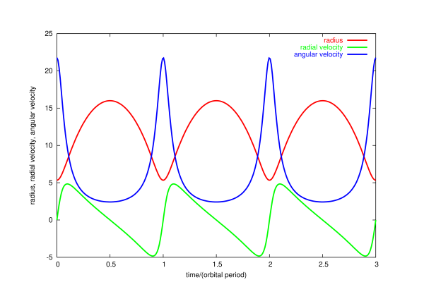
The integral form of Eq.(1.5.44) is

$$\begin{equation} t = \sqrt{\frac{p^3}{GM}} \int \frac{d\phi}{(1+e\cos\phi)^2} + \text{constant}. \tag{1.5.45} \end{equation}$$

This indefinite integral cannot be evaluated in closed form, but it provides a nice way of calculating the orbital period $P$ of bound orbits ($e < 1$). Because this is equal to the time required for $\phi$ to advance by $2\pi$, or twice the time required for $\phi$ to advance by $\pi$, we have

$$P = 2 \sqrt{\frac{p^3}{GM}} \int_0^\pi \frac{d\phi}{(1+e\cos\phi)^2}.$$

This definite integral can be evaluated, and the result is $\pi/(1-e^2)^{3/2}$. We therefore have

$$P = 2\pi \sqrt{\frac{[p/(1-e^2)]^3}{GM}}.$$

We obtain a cleaner form of this result by involving Eq.(1.5.43). In terms of the semi-major axis $a = p/(1-e^2)$, the orbital period is

$$\begin{equation} P = 2\pi \sqrt{\frac{a^3}{GM}}. \tag{1.5.46} \end{equation}$$

We have that $P^2 \propto a^3$, and this is the general statement of Kepler's third law.

1.5.11 Summary

The motion of two bodies subjected to their mutual gravity is described by the relative position vector $\boldsymbol{r} = \boldsymbol{r}_1 - \boldsymbol{r}_2$. When the origin of the coordinate system is at the centre of mass we have

$$\boldsymbol{r}_1 = \frac{m_2}{M} \boldsymbol{r}, \qquad \boldsymbol{r}_2 = -\frac{m_1}{M} \boldsymbol{r}, \qquad M = m_1 + m_2.$$

The vector $\boldsymbol{h} = \boldsymbol{r} \times \boldsymbol{\dot{r}}$ is constant, and $\boldsymbol{h}$ is related to the system's total angular momentum by $\boldsymbol{L} = (m_1 m_2/M) \boldsymbol{h}$. The fact that $\boldsymbol{h}$ is constant implies that the motion takes place in a fixed plane. Using polar coordinates, the motion is described by the functions $r(t)$ and $\phi(t)$. These are determined by the first-order differential equations

$$\frac{1}{2} \dot{r}^2 - \frac{GM}{r} + \frac{h^2}{2r^2} = \varepsilon, \qquad \dot{\phi} = \frac{h}{r^2}.$$

The constant $\varepsilon$ is related to the system's total energy by $E = (m_1 m_2 /M) \varepsilon$. The shape of the orbit is described by

$$r(\phi) = \frac{p}{1 + e\cos\phi}.$$

The orbital elements $(p,e)$ are related to $(h,\varepsilon)$ by

$$h = \sqrt{GMp}, \qquad \varepsilon = -\frac{GM}{p} \bigl(1-e^2\bigr).$$

The motion in time is determined by numerically integrating

$$\dot{\phi} = \sqrt{\frac{GM}{p^3}} (1 + e\cos\phi)^2.$$

When $e < 1$ the motion is elliptical, and the ellipse's semi-major axis is

$$a = \frac{p}{1-e^2}.$$ ,p>The orbital period is then

$$P = 2\pi \sqrt{\frac{a^3}{GM}}.$$

1.6 Appendix: Numerical Integration of Differential Equations

Some of the results presented in this Chapter were obtained by numerical integration. Some of our future results also will be obtained using numerical techniques. In this Appendix we explain the fundamental ideas behind these numerical methods. These ideas are implemented in various available packages, for example, within Maple, or within subroutines found in the book Numerical Recipes.

To begin, we examine a first-order differential equation of the form

$$\begin{equation} \frac{dy}{dx} = f(y), \tag{1.6.1} \end{equation}$$

where $x$ is the independent variable, $y$ the dependent variable, and $f$ an arbitrary function of $y$. A concrete example is

$$\frac{d\phi}{dt} = \sqrt{\frac{GM}{p^3}} (1 + e\cos\phi)^2,$$

which we encountered in Sec.1.5; here $x \equiv t$, $y \equiv \phi$, and $f$ stands for what appears on the right-hand side of the preceding equation.

We seek to determine $y(x)$ in the interval $x_{\rm initial} < x < x_{\rm final}$, starting from the known value $y_{\rm initial}$ at $x = x_{\rm initial}$. The essential idea is to break down the continuum between $x_{\rm initial}$ and $x_{\rm final}$ into a finite number of discrete points separated by a small interval $\Delta$. The computational grid is then

$$\begin{equation} x_n = x_{\rm initial} + n \Delta, \qquad n = 0, 1, 2, \cdots, N, \tag{1.6.2} \end{equation}$$

where $N$ is the total number of points; we have $\Delta = (x_{\rm final} - x_{\rm initial})/N$. Correspondingly, we have the sampled values $y_n = y(x_n)$ of the dependent variable, which we wish to determine. We shall do so by turning the differential equation $dy/dx = f(y)$ into a finite-difference equation.

Consider the first step of moving from $x_0 = x_{\rm initial}$ to $x_1$. We know $y_0 = y_{\rm initial}$, and we wish to determine $y_1$. Because $\Delta$ is small it is safe to assume that the function $f(y)$ changes by very little in the interval between $y_0$ and $y_1$. We may approximate it by its Taylor expansion about $y=y_0$:

$$\begin{align} f(y) &= f(y_0) + f'(y_0) (y-y_0) + \cdots \\ &= f(y_0) \bigl[ 1 + f^{-1} f'(y_0) (y-y_0) + \cdots \bigr]. \end{align}$$

The differential equation gives

$$dx = \frac{dy}{f(y)} = \frac{1}{f(y_0)} \bigl[ 1 - f^{-1} f'(y_0) (y-y_0) + \cdots \bigr]\, dy,$$

where we have used the identity $(1 + \epsilon)^\alpha = 1 + \alpha \epsilon + O(\epsilon^2)$, which holds for any small quantity $\epsilon$ and any power $\alpha$ --- this identity also can be established by Taylor expansion. Integrating the preceding equation gives

$$x_1 - x_0 = \frac{1}{f(y_0)} \Biggl[ (y_1 - y_0) - \frac{1}{2} f^{-1} f'(y_0) (y_1 - y_0)^2 + \cdots \Biggr],$$

or

$$f(y_0) \Delta = (y_1 - y_0) - \frac{1}{2} f^{-1} f'(y_0) (y_1 - y_0)^2 + \cdots.$$

This equation can be solved formally for $y_1 - y_0$:

$$\begin{align} y_1 - y_0 &= f(y_0) \Delta + \frac{1}{2} f^{-1} f'(y_0) (y_1 - y_0)^2 + \cdots \\ &= f(y_0) \Delta + \frac{1}{2} f^{-1} f'(y_0) \bigl[ f(y_0) \Delta + \cdots \bigr]^2 + \cdots f(y_0) \Delta + \frac{1}{2} f f'(y_0) \Delta^2 + \cdots. \end{align}$$

We write this result as

$$\begin{equation} y_1 = y_0 + f(y_0) \Delta + \frac{1}{2} f f'(y_0) \Delta^2 + O(\Delta^3), \tag{1.6.3} \end{equation}$$

indicating that the error of this approximation for $y_1$ is of order $\Delta^3$ and therefore quite small.

A cruder approximation for $y_1$ is

$$y_1 = y_0 + f(y_0) \Delta + O(\Delta^2),$$

and this approximation is at the core of Euler's method to solve the differential equation: From the known value $y_0$ compute $f(y_0)$ and multiply by $\Delta$; add the result to $y_0$ to get $y_1$, and repeat the procedure to get $y_2$, $y_3$, and so on. Euler's method is very simple and economical, but because its error term is of order $\Delta^2$, it is not very accurate. With a little cleverness, however, it is possible to improve the accuracy of the method so that its error term becomes of order $\Delta^3 \ll \Delta^2$. One way of achieving this would be to use Eq.(1.6.3) instead of its cruder version. The price to pay would be the need to evaluate $f'(y)$, the derivative of the function with respect to $y$. This may not be practical in some circumstances, and there is an alternative method.

Consider evaluating the function $f$ not at $y=y_0$, but at the midpoint between $y_0$ and $y_1 \simeq y_0 + f(y_0) \Delta$:

$$f(y_0) \to f(y_0 + {\textstyle \frac{1}{2}} f_0 \Delta),$$

where we use the notation $f_0 = f(y_0)$. By Taylor expansion we have

$$\begin{align} f(y_0 + {\textstyle \frac{1}{2}} f_0 \Delta) &= f(y_0) + f'(y_0) ({\textstyle \frac{1}{2}} f_0 \Delta) + O(\Delta^2) \\ &= f(y_0) + \frac{1}{2} f f'(y_0) \Delta + O(\Delta^2), \end{align}$$

and this shows that Eq.(1.6.3) is equivalent to

$$\begin{equation} y_1 = y_0 + f(y_0 + {\textstyle \frac{1}{2}} f_0 \Delta) \Delta + O(\Delta^3). \tag{1.6.4} \end{equation}$$

This approximation for $y_1$ has an error term of order $\Delta^3$, and it is obtained simply by evaluating the function $f$ at the midpoint; the value of its derivative is not needed.

By being increasingly clever it is possible to decrease further the size of the error term. The fourth-order Runge-Kutta method consists of the following recipe. Suppose that the differential equation has been integrated up to $x = x_n$, and that we wish to proceed to the next grid point, at $x = x_{n+1}$. We have therefore obtained $y_n$ and we wish to calculate $y_{n+1}$. First we compute the auxiliary quantities

$$\begin{align} k_1 &= f(y_n) \Delta, \\ k_2 &= f(y_n + {\textstyle \frac{1}{2}} k_1) \Delta, \\ k_3 &= f(y_n + {\textstyle \frac{1}{2}} k_2) \Delta, \\ k_4 &= f(y_n + k_3) \Delta, \end{align}$$

and next we approximate $y_{n+1}$ by

$$\begin{equation} y_{n+1} = y_n + \frac{1}{6} k_1 + \frac{1}{3} k_2 + \frac{1}{3} k_3 + \frac{1}{6} k_4 + O(\Delta^5). \tag{1.6.5} \end{equation}$$

As indicated, the judicious choice of coefficients in front of $k_1$, $k_2$, $k_3$, and $k_4$ ensures that the error term is now of order $\Delta^5$, and therefore very small. The Runge-Kutta method is easy to implement, it is accurate, and it is robust; it works well for most functions $f(y)$. The method can also be generalized to handle functions $f(x,y)$ that depend on both variables.

The method also generalizes to a set of differential equations

$$\begin{equation} \frac{d y[i]}{dx} = f[i]\bigl(y[1],y[2],\cdots\bigr), \qquad i = 1, 2, \cdots \tag{1.6.6} \end{equation}$$

for a set of dependent variables $y[i]$. In this case the auxiliary quantities $k_1$, $k_2$, $k_3$, and $k_4$ acquire an index $[i]$; for example we now have

$$k_1[i] = f[i]\bigl( y_n[1], y_n[2], \cdots \bigr) \Delta$$

and

$$k_2[i] = f[i]\bigl( y_n[1] + {\textstyle \frac{1}{2}} k_1[1], y_n[2] + {\textstyle \frac{1}{2}} k_1[2], \cdots) \Delta.$$

This generalization is useful, because it allows us to use the method to integrate second-order differential equations. Consider, for example, the pendulum equation of Eq.(1.3.25),

$$\ddot{\theta} + \omega^2 \sin\theta = 0.$$

This can be recast as a system of two first-order differential equations. To do this we define $y[1] = \theta$ and $y[2] = \dot{\theta}$. When then have the system

$$\begin{align} \frac{dy[1]}{dt} &= y[2], \\ \frac{dy[2]}{dt} &= -\omega^2 \sin(y[1]). \end{align}$$

In this instance we find that $f[1](y[1],y[2]) = y[2]$ and $f[2](y[1],y[2]) = -\omega^2 \sin(y[1])$. This system of equations can be integrated straightforwardly, and the result for $y[1](t)$ is the numerical approximation to $\theta(t)$, the solution to the original second-order equation.

1.7 Problems

1. Let

   $$\boldsymbol{A} = (3x^2 - 6yz) \boldsymbol{\hat{x}} + (2y+3xz) \boldsymbol{\hat{y}} + (1-4xyz^2) \boldsymbol{\hat{z}}.$$

   Calculate $\int_C \boldsymbol{A} \cdot d\boldsymbol{s}$ along the following paths that link the point $(0,0,0)$ to the point $(1,1,1)$:

   a) The curve described by $x=u$, $y=u^2$, and $z=u^3$, in which the parameter $u$ is restricted to the interval $0 < u < 1$.

   b) The straight line that joins these points.

2. Let

   $$\boldsymbol{A} = (2xy+z^3) \boldsymbol{\hat{x}} + (x^2+2y) \boldsymbol{\hat{y}} + (3x z^2 - 2) \boldsymbol{\hat{z}}.$$

   Find the function $f$ such that $\boldsymbol{A} = \boldsymbol{\nabla} f$. Then evaluate $\int_C \boldsymbol{A} \cdot d\boldsymbol{s}$ along any path $C$ that links the point $(1,-1,1)$ to the point $(2,1,2)$.

3. Evaluate $\oint_C \boldsymbol{r} \cdot d\boldsymbol{s}$ along all closed loops $C$, where $\boldsymbol{r} = x \boldsymbol{\hat{x}} + y \boldsymbol{\hat{y}} + z \boldsymbol{\hat{z}} is the position vector.

4. A projectile is launched with initial speed $v_0$ at an angle $\alpha$ with the horizontal. Calculate:

   a) the position vector as a function of time;

   b) the time required to reach the highest point;

   c) the maximum height reached by the projectile;

   d) the time of flight back to the Earth's surface;

   e) the range of the projectile;

   f) the angle $\alpha$ which maximizes the range.

5. Suppose that in the preceding problem, the projectile is also subjected to a frictional force equal to $-k \boldsymbol{v}$, where $\boldsymbol{v}$ is the velocity vector and $k$ a positive constant. Find:

   a) the velocity vector as a function of time;

   b) the position vector as a function of time;

   c) the terminal velocity of the projectile.

   For ease of notation set $k = m/\tau$.

6. A particle of mass $m$ is traveling in the $x$ direction. At time $t = 0$ it is located at $x = 0$ and has a speed $v_0$. The particle is subjected to a frictional force which opposes the motion; its magnitude is equal to $\beta v^2$, where $v = v(t)$ is the particle's speed at time $t$ and $\beta$ is a positive constant.

   a) What is the speed of the particle as a function of time?

   b)What is the position of the particle as a function of time?

7. A particle of mass $m$ rests on top of a sphere of radius $R$. The particle is then displaced slightly so that it starts to move down the sphere. (It is assumed that the particle slides down without rolling and without friction.) As it moves down the sphere, the particle makes an angle $\theta$ with the vertical direction. At some point the particle loses contact with the surface of the sphere, and it proceeds to fall freely. We are interested in the motion of the particle from the initial moment where it is at rest to the final moment where it leaves the sphere.

   a) Derive an equation of motion for $\theta(t)$, and find an expression for $N$, the magnitude of the normal force.

   b) At which angle $\theta$ does the particle leave the surface of the sphere?

   c) What is the speed of the particle when it leaves the surface of the sphere?

   [Hint: This problem is involved. You may find it useful to resolve the force and acceleration vectors into a basis that consists of $\boldsymbol{\hat{r}}$, a unit vector that points in the direction normal to the sphere, and $\boldsymbol{\hat{\theta}}$, a unit vector that points in the direction of increasing $\theta$.]

8. The planar pendulum of Sec.1.3.7 is now subjected to a frictional force $\boldsymbol{F}_{\rm friction} = -(m/\tau) \boldsymbol{v}$, where $\tau$ is a positive constant. Derive the new equation of motion for the swing angle $\theta$.

9. The equation of motion of the preceding problem reduces to

   $$\ddot{\theta} + 2\gamma \dot{\theta} + \omega^2\theta = 0$$

   when the oscillations have a very small amplitude; here $\gamma$ is a positive constant that is related to $\tau$ in the preceding problem. Find the general solution to this equation. Assume that $\omega^2 > \gamma^2$, so that the oscillations are underdamped. [Be sure that your final expression for $\theta(t)$ is a real (not complex) function.]

10. A mass $m$ is allowed to move along the $x$ axis, either in the positive or in the negative direction. It is subjected to a constant force $+F$ when $x < 0$ and to a constant force $-F$ when $x > 0$ (here $F$ is positive).

    a) Describe the motion qualitatively with the help of an energy diagram.

    b) Calculate the period of the motion; express your result in terms of $m$, $F$, and the amplitude $A$ of the motion.

11. A cylindrical cork is partially immersed in a liquid of (mass) density $\rho$. The cork's axis is oriented with the vertical direction, and the cork floats in the liquid. The cylinder's cross-sectional area is $A$, and its mass is $m$. The cork is gently pushed down into the liquid and then released; it starts to oscillate. Neglecting any damping effect, calculate the angular frequency $\omega$ of the oscillations.

    [Hint: The restoring force is provided by the buoyancy of the liquid. According to the Archimedes principle, the buoyant force is equal to the weight of the liquid displaced by the cork.]

12. For Kepler's problem, prove that the square of the velocity vector $\boldsymbol{v} = \boldsymbol{\dot{r}}$ can be expressed as

    $$v^2 = GM \biggl( \frac{2}{r} - \frac{1}{a} \biggr),$$

    where $a = p/(1-e^2)$ is the ellipse's semi-major axis. What is $v$ at pericentre? What is $v$ at apocentre? (Express your results in units of the average speed $\bar{v} = \sqrt{GM/a}$.)

13. We have seen that the description of Keplerian motion in time can be obtained by integrating Eq.~(1.4.52). An alternative method is based on the representation

    $$r = a(1 - e\cos\psi),$$

    in which $r$ is expressed in terms of the eccentric anomaly $\psi$; this is an angular parameter that ranges from 0 to $2\pi$ as each body completes one full orbit. We wish to find $\psi$ as a function of time.

    a) Starting from the statement of energy conservation, $\frac{1}{2} \dot{r}^2 + \nu(r) = \varepsilon$, in which you are to substitute $h^2 = GMa(1-e^2)$ and $\varepsilon = -GM/(2a)$, derive an expression for $\dot{\psi}$. Make sure that this expression is simplified to the full extent possible.

    b) Integrate the equation for $\dot{\psi}$ that was obtained in part (a). Show that the solution is

    $$\psi - e \sin\psi = \sqrt{\frac{GM}{a^3}} \bigl( t - t_0 \bigr),$$

    where $t_0$ is the time at which $\psi = 0$. This is Kepler's equation, and it can be numerically inverted to yield $\psi(t)$. This method is the most convenient to find the behaviour of $r$ as a function of time.

14. We examine a special case of Kepler's problem. We set $h=0$, so that $\dot{\phi} = 0$. We have purely radial motion, and the equation for $r(t)$ reduces to

    $$\frac{1}{2} \dot{r}^2 - \frac{GM}{r} = \varepsilon,$$

    where $\varepsilon$ is the reduced total energy.

    a) Construct an energy diagram for this situation. Describe the motion qualitatively when $\varepsilon > 0$, when $\varepsilon = 0$, and when $\varepsilon < 0$.

    In the rest of the problem we consider the subcase $\varepsilon < 0$ in some detail.

    b) Relate $\varepsilon$ to $r_{\rm max}$, the maximum value of $r$ at which a turning point occurs.

    c) Imagine that the motion proceeds from $r=r_{\rm max}$ to  $r=0$. We represent this mathematically in terms of an auxiliary variable, the angle $\eta$. We write

    $$r(\eta) = \frac{1}{2} r_{\rm max} (1 + \cos\eta),$$

    and we let $\eta$ vary from $\eta = 0$ to $\eta = \pi$. Calculate $\dot{\eta} = d\eta/dt$ and solve this for $t(\eta)$. The motion is now completely determined. Provide a plot of $r$ as a function of $t$.

    d) What is the total time required for the bodies to go from $r = r_{\rm max}$ to $r = 0$?

15. Two particles move about each other in circular orbits under the influence of their gravitational attraction; their orbital period is $\tau$. Their motion is suddenly stopped at a given instant of time, and they are then released and allowed to fall into each other. Calculate the time required for them to collide; express your answer in terms of $\tau$.

    [Hint: You will need the result of part (d) of the preceding problem.]

16. The escape velocity of a particle on Earth is the minimum velocity required on the Earth's surface for the particle to escape the Earth's gravitational field. Neglecting air resistance within the atmosphere, calculate this in terms of the Earth's mass $M$ and its radius $R$. Evaluate this numerically and show that it is close to 11 km/s.

17. Two bodies of mass $m_1$ and $m_2$ are subjected to their mutual forces, so that the force acting on body 1 due to body 2 is $\boldsymbol{F}_{12} = -f(r) \boldsymbol{\hat{r}}$, while the force acting on body 2 due to body 1 is $\boldsymbol{F}_{21} = +f(r) \boldsymbol{\hat{r}}$. Here $f$ is an arbitrary function of $r = |\boldsymbol{r}_1 - \boldsymbol{r}_2|$, the distance between the bodies, and the forces are directed along $\boldsymbol{\hat{r}} = \boldsymbol{r}/r$, where $\boldsymbol{r} = \boldsymbol{r}_1 - \boldsymbol{r}_2$; such forces are called central forces.

    a) Derive an equation of motion for $\boldsymbol{R}$, the position of the centre of mass.

    b) Derive an equation of motion for $\boldsymbol{r}$, the position of body 1 relative to body 2.

    c) Prove that $\boldsymbol{h} = \boldsymbol{r} \times \boldsymbol{\dot{r}}$ is a constant vector; conclude that the motion takes place in a fixed plane.

    d) Introduce the polar coordinates $(r,\phi)$ and prove that $|\boldsymbol{h}| = h = r^2 \dot{\phi}$; conclude that Kepler's law --- the law of areas --- is valid for all central forces, and not just for gravity.

    e) Show that the equation of motion for $r$ reduces to

    $$\ddot{r} + \frac{f}{\mu} - \frac{h^2}{r^3} = 0,$$

    where $\mu = m_1 m_2/(m_1 + m_2)$ is known as the reduced mass of the two-body system.

    f) Prove that the shape of the orbit is determined by

    $$\frac{d^2 u}{d\phi^2} + u = \frac{f}{\mu h^2 u^2},$$

    where $u = 1/r$.

18. A central force $f = k/r^n$, where $k$ is a constant and $n$ an integer, is known to produce an orbit described by $r = a e^{-\phi}$, where $a$ is a constant.

    a) Plot this orbit in the $x$-$y$ plane.

    b) Determine the integer $n$.

19. A central force $f = k/r^n$, where $k$ is a constant and $n$ an integer, is known to produce an orbit described by $r = a \sqrt{\cos2\phi}$, where $a$ is a constant.

    a) Plot this orbit in the $x$-$y$ plane.

    b) Determine the integer $n$.

20. A two-body system moves under the influence of a central force given by

    $$f = \frac{a}{r^2} + \frac{b}{r^3},$$

    where $a$ and $b$ are constants.

    a) Show that the shape of the orbit is described by

    $$r = \frac{p}{1 + e \cos(k\phi)},$$

    where $p$, $e$, and $k$ are constants. Express $p$ and $k$ in terms of $a$, $b$, $h^2$, and $\mu$. (Assume that $b < \mu h^2$.)

    b) Plot the orbit in the $x$-$y$ plane. Set $p=1$, $e=0.6$, $k=0.99$, and let $\phi$ range from 0 to $16\pi$. What is happening to the major axis of the ellipse?

1.8 Additional Problems

1. An inclined plane makes an angle $\alpha$ with the horizontal. A projectile is launched from point $A$ at the bottom of the inclined plane. Its initial speed is $v_0$, and its initial velocity vector makes an angle $\beta$ with the horizontal. The projectile eventually hits the inclined plane at point $B$. Air resistance is negligible.

   a) Calculate the range $R$ of the projectile, the distance between points $A$ and $B$. Show that it it can be expressed in the form

   $$R = R_0 \sin(\beta-\alpha) \cos\beta$$

   and find an expression for $R_0$.

   b) Find the angle $\beta_{\rm max}$ which maximizes the range.

2. A particle traveling in the positive $x$ direction is subjected to a force $F = k x^3$. The particle started from an initial position $x_0 < 0$. Draw an energy diagram for this situation and provide a qualitative description of the possible motions.

3. Two bodies of masses $m_1$ and $m_2$ are subjected to a mutual attractive force $\boldsymbol{F}_{12} = -k m_1 m_2 \boldsymbol{r}$, where $k$ is a constant and $\boldsymbol{r} = \boldsymbol{r}_1 - \boldsymbol{r}_2$ is the relative position vector.

   a) Show that the equation of motion for $r(t)$ can be put in the form of an energy equation,

   $$\frac{1}{2} \dot{r}^2 + \nu(r) = \varepsilon,$$

   and find an expression for $\nu(r)$, the effective potential. Draw an energy diagram for this system and give a qualitative description of the possible motions.

   b) Prove that

   $$r(\phi) = \frac{r_0}{\sqrt{2 - e - e\cos(2\phi)}}$$

   describes the shape of the orbit, and solve for $r_0$ in terms of theconstants $e$, $M = m_1 + m_2$, $h$, and $k$.

4. The parabolic coordinates $u$ and $v$ are sometimes useful to describe the motion of a particle in a two-dimensional plane. These are related to the Cartesian coordinates $x$ and $y$ by

   $$x = uv, \qquad y = \frac{1}{2} (u^2 - v^2).$$

   a) Sketch the shapes of the curves $u =\text{constant}$ in the $x$-$y$ plane.

   b) Sketch the shapes of the curves $v =\text{constant}$ in the $x$-$y$ plane.

   c) Find the unit vectors $\boldsymbol{\hat{u}}$ and $\boldsymbol{\hat{v}}$ associated with this coordinate system.