Chapter 2: Lagrangian Mechanics
Equations will not display properly in Safari-please use another browser
2.1 Introduction: From Newton to Lagrange
The methods of Newtonian mechanics, based on the vectorial equation $\boldsymbol{F} = m \boldsymbol{a}$, are very powerful and they can be applied to all mechanical systems. But they lack in efficiency when Cartesian coordinates $(x,y,z)$ do not give the simplest description of a mechanical system. An example is the problem of the pendulum (Sec.1.3.7), which is best analyzed in terms of the swing angle $\theta$; we have seen that to derive the equation of motion for $\theta(t)$ requires somewhat laborious calculations, and the reason is precisely that $\theta$ is not a Cartesian coordinate. Another example is Kepler's problem (Sec.1.5), which is best analyzed in terms of the polar coordinates $(r,\phi)$; again we saw (back in Sec.1.5.4) that to derive equations of motion for $r(t)$ and $\phi(t)$ required some long calculations.
To increase the efficiency of the theoretical methods of mechanics, a number of scientists in the centuries following Newton endeavoured to recast the Newtonian laws into a more flexible formulation. The most famous players include Leonhard Euler (1707--1783), Joseph Lagrange (1736--1813), William Rowan Hamilton (1805--1865), and Carl Gustav Jacobi (1804--1851). Their new techniques proved extremely useful, and they allowed them and others to solve increasingly challenging problems, most notably in the context of celestial mechanics. These new powerful techniques are the topic of this chapter on Lagrangian mechanics, and the following chapter on Hamiltonian mechanics.
It is important to point out that the Lagrangian and Hamiltonian formulations of the laws of mechanics are largely restricted to forces that can be derived from a potential. For other problems, such as a particle subjected to air resistance, the new techniques cannot be applied in a very straightforward way, and it is usually best to go back to the old Newtonian methods. In this chapter and the next, we shall consider only forces that can be derived from a potential.
The entire content of Lagrangian mechanics is summarized in the following simple recipe:
-
Select generalized coordinates $q_a$ to describe the degrees of freedom of a mechanical system. These coordinates are completely arbitrary. They need not be the original Cartesian coordinates associated with an inertial frame. Indeed, there is no need for the coordinates to even be attached to an inertial frame. The index $a = 1, 2, \cdots$ labels each one of the generalized coordinates; there is one coordinate for each degree of freedom.
-
In terms of the generalized coordinates, calculate the system's total kinetic energy $T$ and total potential energy $V$. Then form what is known as the Lagrangian function of the system, which is denoted $L(q_a,\dot{q}_a)$; this depends on the generalized coordinates $q_a$ and the generalized velocities $\dot{q}_a = dq_a/dt$. The Lagrangian is defined by
\[L = T - V;\]
it is the difference between the kinetic and potential energies.
-
Substitute the Lagrangian into the Euler-Lagrange (EL)
equations,
\[\frac{d}{dt} \frac{\partial L}{\partial \dot{q}_a} -\frac{\partial L}{\partial q_a} = 0.\]
This returns an equation of motion for each generalized coordinate $q_a(t)$. There is one EL equation for each generalized coordinate.
-
The rest of the recipe is concerned with solving the equations of motion. The methods for doing this are varied, and they depend on the particular situation, just as they do in the Newtonian formulation.
Let us first verify that the recipe is compatible with Newton's laws. Consider a particle moving in three-dimensional space and subjected to a potential $V(x,y,z)$. As indicated, we use Cartesian coordinates to describe the motion of the particle. In this case, therefore, the generalized coordinates are chosen as $q_1 = x$, $q_2 = y$, and $q_3 = z$. The particle's kinetic energy is $T = \frac{1}{2} m (\dot{x}^2 + \dot{y}^2 + \dot{z}^2)$, and the Lagrangian function is
\[ L(x,y,z,\dot{x},\dot{y},\dot{z}) = \frac{1}{2} m (\dot{x}^2 + \dot{y}^2 + \dot{z}^2) - V(x,y,z). \]
To substitute this into the EL equation for $q_1 = x$, say, we must first evaluate $\partial L/\partial \dot{x}$. This is the derivative of $L$ with respect to $\dot{x}$, treating all other variables (including $x$) as constant parameters. This is given by
\[ \frac{\partial L}{\partial \dot{x}} = m \dot{x}. \]
We next differentiate this with respect to $t$, and get
\[ \frac{d}{dt} \frac{\partial L}{\partial \dot{x}} = m \ddot{x}. \]
Finally, we differentiate $L$ with respect to $x$, treating all other variables (including $\dot{x}$) as constant parameters; this gives
\[ \frac{\partial L}{\partial x} = - \frac{\partial V}{\partial x}. \]
Substituting these results into the EL equation for $x$, we arrive at
\[ m \ddot{x} + \frac{\partial V}{\partial x} = 0. \]
Repeating these calculations for $y$ and $z$ would eventually return the full vectorial equation
\[ m \boldsymbol{a} + \boldsymbol{\nabla} V = \boldsymbol{0}, \]
or $m \boldsymbol{a} = \boldsymbol{F}$ if we recall that the force is derived from the potential, so that $\boldsymbol{F} = -\boldsymbol{\nabla} V$. This exercise reveals that indeed, the Lagrangian recipe is compatible with the Newtonian law.
The true power of the recipe, however, is revealed when the generalized coordinates are not Cartesian. Let us see what the recipe produces in the case of the pendulum. Recall from Sec.~\ref{i.3.7} that the pendulum's single degree of freedom is best represented by the swing angle $\theta$; this will be our generalized coordinate for this problem, and we write $q \equiv \theta$. (We do not need a label $a$ in this case, as there is only one generalized coordinate.) The relation between $\theta$ and the original Cartesian coordinates is $x = \ell \sin\theta$ and $z = \ell \cos\theta$, with $\ell$ denoting the length of the rod. The pendulum's kinetic energy is $T = \frac{1}{2} (\dot{x}^2 + \dot{z}^2) = \frac{1}{2} m \ell^2 \dot{\theta}^2$. Its potential energy is $V = -mgz = -mg\ell\cos\theta = -m\ell^2 \omega^2 \cos\theta$, where we have reintroduced the quantity $\omega^2 \equiv g/\ell$. The pendulum's Lagrangian function is
\[ L(\theta,\dot{\theta}) = m\ell^2 \biggl( \frac{1}{2} \dot{\theta}^2 + \omega^2 \cos\theta \biggr). \]
To substitute this into the EL equation we must first evaluate $\partial L/\partial \dot{\theta}$, the partial derivative of $L$ with respect to $\dot{\theta}$. This is
\[ \frac{\partial L}{\partial \dot{\theta}} = m\ell^2 \dot{\theta}. \]
Next we differentiate this with respect to time, and obtain
\[ \frac{d}{dt} \frac{\partial L}{\partial \dot{\theta}} = m\ell^2 \ddot{\theta}. \]
Finally we calculate the partial derivative of $L$ with respect to $\theta$, which yields
\[ \frac{\partial L}{\partial \theta} = -m\ell^2 \omega^2 \sin\theta. \]
Substituting these results into the EL equation produces
\[ m\ell^2 \bigl( \ddot{\theta} + \omega^2 \sin\theta \bigr) = 0, \]
the same pendulum equation as in Eq.(1.3.25). Comparing the computations carried out here to those required in Sec.1.3.7, the greater efficiency of the Lagrangian recipe should come out loud and clear.
It is possible to derive the Lagrangian recipe from Newton's law, $\boldsymbol{F} = m \boldsymbol{a}$. The derivation is fairly laborious, and it involves performing a transformation from the original Cartesian system $(x,y,z)$ to the generalized coordinates $q_a$. It is possible, however, and more interesting, to derive the recipe from a new physical principle. Instead of postulating the validity of $\boldsymbol{F} = m\boldsymbol{a}$ as the starting point of Newtonian mechanics, we shall instead adopt the principle of least action as the starting point of Lagrangian mechanics. As we shall see in the next two sections, the Euler-Lagrange equations can be derived as a direct consequence of the principle of least action, and as we have already seen, these are fully compatible with Newton's law. What we have, therefore, is the Newtonian postulate arising as a consequence of the new principle. More importantly, we have the more flexible framework of the EL equations arising as a consequence of the principle of least action.
As we shall see below, the principle of least action states that of all the possible paths $q_a(t)$ that a mechanical system could take to go from configuration 1 to configuration 2, the paths that are actually taken are the ones which minimize the system's action functional, defined by
\[ S[q_a(t)] = \int_{t_1}^{t_2} L(q_a,\dot{q}_a)\, dt. \]
This beautiful statement is mathematically equivalent to the full set of EL equations, which give rise to the equations of motion that determine the actual paths of the system. This formulation of the laws of mechanics, in terms of a least-action principle, is economical and conceptually compelling. It is also extremely powerful: Virtually all fundamental laws of physics (including field theories) can be formulated in terms of such an action principle.
2.2 Calculus of Variations
In this section we introduce the mathematical tools --- the calculus of variations --- that are required in the derivation of the Euler-Lagrange (EL) equations from the principle of least action. We will look at this issue from a purely mathematical point of view, and return to the physics in the next section.
2.2.1 Curve of Maximum Area
Let us examine the following mathematical problem. We consider the infinite number of curves in the $x$-$y$ plane that link the point $(x=-1,y=0)$ to the point $(x=+1,y=0)$; see Fig.2.1. Of all these curves we select those that have a total arc length (the total distance traveled along the curve) equal to $\pi$. Of all the curves that are left we wish to find the one which maximizes the area under the curve. (Notice that the mathematical problem involves maximization of an area, while the physical problem involves minimization of an action. The mathematical techniques to be developed below work for both cases, maximization and minimization, and they do not care about the identity of the quantity to be extremized.)
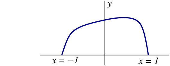
We describe the family of curves introduced in the previous paragraph by parametric relations $x(s)$ and $y(s)$, in which the parameter $s$ is the curve's arc length, calculated from the starting point $(-1,0)$. Because all the curves within the family have a total arc length of $\pi$, the parameter $s$ ranges from $0$ to $\pi$ as each curve runs from $(-1,0)$ to $(+1,0)$. We have $ds^2 = dx^2 + dy^2$, and this relation implies that the functions $x(s)$ and $y(s)$ are not independent of each other. The area under the curve is obtained by integration, $A = \int y\, dx$, which we write as
\[ A = \int_0^\pi y(s) \frac{dx}{ds}\, ds. \]
We can replace the factor $dx/ds$ by $\sqrt{1 - y^{\prime 2}}$, where $y' = dy/ds$. This gives us, finally,
\begin{equation} A = \int_0^\pi y \sqrt{ 1 - y^{\prime 2} }\, ds. \tag{2.2.1} \end{equation}
We wish to find the function $y(s)$ that produces the largest possible value for $A$. Once this function is identified, $x(s)$ can be obtained by integrating the equation
\begin{equation} x' = \sqrt{ 1 - y^{\prime 2} }. \tag{2.2.2} \end{equation}
The maximal curve is then fully determined.
2.2.2 Extremum of a Functional
To proceed it is helpful to broaden the scope of the preceding discussion and to examine the general structure of the mathematical problem. We are given a functional $A[y]$, a function $A$ of a function $y(s)$, which we wish to maximize, or perhaps minimize, with respect to the choice of path $y(s)$. (In general we say that we wish to find the extremum of the functional, and we shall never need to distinguish between a maximum and a minimum.) The functional has the following structure:
\begin{equation} A[y] = \int_{s_0}^{s_1} G(y,y')\, ds; \tag{2.2.3} \end{equation}
it is given by an integral over a parameter $s$ of a function $G$ which depends on the path $y(s)$ and its derivative $y'(s) = dy/ds$. The integral can be evaluated for any choice of trial function $y_{\rm trial}(s)$, and the result is a number $A_{\rm trial}$. We are looking for the function $\bar{y}(s)$ that produces the largest (or smallest) number. In mathematical terms, we are looking for the extremum of the functional $A[y]$.
The mathematical task of extremizing a function $f(x)$ with respect to its argument $x$ --- the argument being a number --- is a simple one: We simply calculate the derivative of the function and set the result equal to zero; the solutions to $df/dx = 0$ are all extremum points (minima and maxima) of the function. To extremize a functional $A[y]$ with respect to a functional argument $y(s)$ is a much more delicate task. How does one do this?
Let us examine more closely the straightforward task of finding an extremum of a function $f(x)$. We imagine, for concreteness, that the function has a single maximum at $x = \bar{x}$; this is represented in Fig.2.2. We have, of course, $f'(\bar{x}) = 0$, with a prime indicating differentiation with respect to $x$.
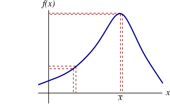
An important property of $\bar{x}$ is that it is the point from which the function $f(x)$ changes the least when $x$ is displaced from $\bar{x}$ to a neighbouring point $\bar{x} + \delta x$. That this is so can easily be seen from the figure, but it is just as easy to prove it mathematically. Let us calculate $\delta f$, the change induced in the function when its argument $x$ is moved to a neighbouring point $x + \delta x$. By Taylor's theorem we have
\begin{align} \delta f &\equiv& f(x + \delta x) - f(x) // &= f'(x) \delta x + \frac{1}{2} f''(x) (\delta x)^2 + \cdots. \end{align}
From this calculation we learn that in general, the change in the function is proportional to $\delta x$, as we might have expected. But when we let $x$ become an extremum point $\bar{x}$, we get a different result. In this case we have $f'(\bar{x}) = 0$ and the preceding equation becomes
\[ \delta f = \frac{1}{2} f''(\bar{x}) (\delta x)^2 + \cdots. \]
Now the change in the function is proportional to $(\delta x)^2$, and this is much smaller than what we get in the general case. We have just found that the variation $\delta f$ is smallest when it is taken at an extremum point. A useful way of characterizing an extremum point is therefore to say that it is a point from which a displacement $\delta x$ produces a vanishing change $\delta f$, to linear order in $\delta x$. (The change is not actually zero, but it is of second order in $\delta x$, as we have shown.)
We shall use the same idea to find the extremum path of a functional. We will look for a path $\bar{y}(s)$ --- analogous to the extremum point $\bar{x}$ --- that has the property that a displacement away from this path produces no change in the functional $A[y]$, to linear order in the displacement $\delta y(s)$. In other words, if we evaluate the function on the extremum path $\bar{y}(s)$ and get the number $\bar{A}$, we will find that if we then evaluate the functional on the displaced path $y(s) = \bar{y}(s) + \delta{y}(s)$, we will still get the number $\bar{A}$, except for a correction of second order in the displacement; the change $\delta A$ is zero to first order in $\delta y(s)$.
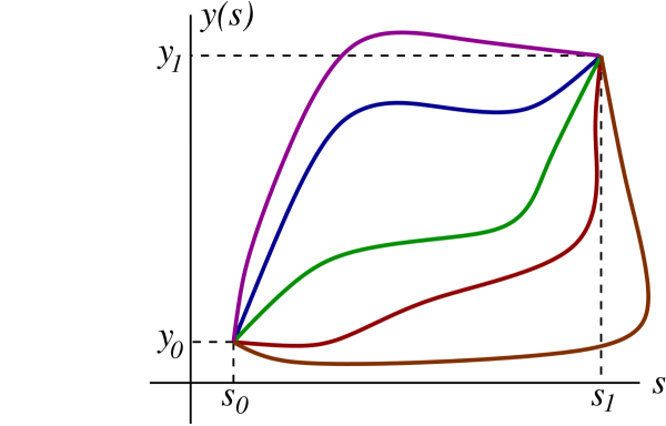
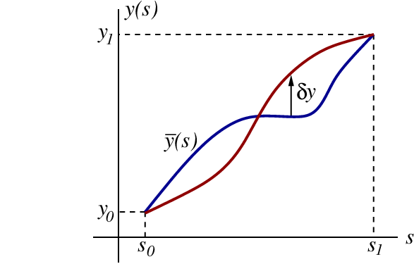
To flesh this out let us consider all paths $y(s)$ that leave the point $y = y_0$ when $s = s_0$ and arrive at the point $y = y_1$ when $s = s_1$; members of this family of curves are displayed in Fig.2.3. Out of all these possible paths that link $y_0$ and $y_1$ we wish to find the one which extremizes the functional $A[y]$. Our strategy will be to assume the existence of an extremum path, which we denote $\bar{y}(s)$, and which we treat as a reference path. We shall examine what happens to $A[y]$ when we displace the path from $y(s) = \bar{y}(s)$ to $y(s) = \bar{y}(s) + \delta y(s)$. While we shall find that in general, this produces a change $\delta A$ that is proportional to $\delta y(s)$, we will instead demand that $\delta A$ vanish to first order in the displacement; as we shall see, this procedure will permit us to identify the extremum path $\bar{y}(s)$. To carry out this procedure properly it is important to ensure that all the considered paths begin and end at the same two end points. The reference path $\bar{y}(s)$ and the displaced paths $y(s) = \bar{y}(s) + \delta y(s)$ must all satisfy $y(s_0) = y_0$ and $y(s_1) = y_1$. This implies that the displacement $\delta y(s)$, which are completely arbitrary in the interval $s_0 < s < s_1$, must satisfy the boundary conditions
\begin{equation} \delta y(s_0) = 0 = \delta y(s_1). \tag{2.2.4} \end{equation}
The situation is illustrated in Fig.2.4.
We evaluate first the functional $A[y]$ on the reference path $\bar{y}(s)$; this is
\[ \bar{A} = A[\bar{y}] = \int_{s_0}^{s_1} G(\bar{y},\bar{y}')\, ds. \]
We next evaluate the functional on a displaced path $y(s) = \bar{y}(s) + \delta y(s)$; this is
\[ A[\bar{y}+\delta y] = \int_{s_0}^{s_1} G(\bar{y}+\delta y,\bar{y}' + \delta y')\, ds, \]
where $\delta y' \equiv y' - \bar{y}' = d(y-\bar{y})/ds = d(\delta y)/ds$. The change in the functional is
\begin{align} \delta A &= A[\bar{y}+\delta y] - A[\bar{y}] \\ &= \int_{s_0}^{s_1} \Bigl[G(\bar{y}+\delta y,\bar{y}' + \delta y') - G(\bar{y},\bar{y}') \Bigr]\, ds, \end{align}
and we wish to find conditions on $\bar{y}(s)$ that will allow us to set $\delta A = 0$, up to corrections of second order in $\delta y$.
The function $G$ depends on two variables, $y(s)$ and $y'(s)$. By Taylor's theorem we have
\[ G(\bar{y}+\delta y,\bar{y}' + \delta y') = G(\bar{y},\bar{y}') + \frac{\partial G}{\partial y} \biggr|_{y=\bar{y}, y'=\bar{y}'} \delta y + \frac{\partial G}{\partial y'} \biggr|_{y=\bar{y}, y'=\bar{y}'} \delta y' + \cdots, \]
where we omit terms of higher order than first in the displacements $\delta y(s)$ and $\delta y'(s)$. The change in functional is therefore
\[ \delta A = \int_{s_0}^{s_1} \biggl[ \frac{\partial G}{\partial y}\, \delta y + \frac{\partial G}{\partial y'}\, \delta y' \biggr]\, ds, \]
where we again neglect higher-order terms, and where we discard the signs $|_{y=\bar{y}, y'=\bar{y}'}$ that instruct us to evaluate the partial derivatives on the reference path $\bar{y}(s)$; this operation will henceforth be understood.
Recalling that $\delta y' = d(\delta y)/ds$, we manipulate the second term within the integral:
\begin{align} \frac{\partial G}{\partial y'}\, \delta y'\, ds &= \frac{\partial G}{\partial y'}\, d (\delta y) \\ &= d \biggl(\frac{\partial G}{\partial y'}\, \delta y \biggr) - \delta y\, d \biggl(\frac{\partial G}{\partial y'} \biggr) \\ &= d \biggl(\frac{\partial G}{\partial y'}\, \delta y \biggr) - \delta y\, \frac{d}{ds} \frac{\partial G}{\partial y'}\, ds. \end{align}
This term can be integrated by parts, and we obtain
\[ \delta A = \frac{\partial G}{\partial y'}\, \delta y \biggr|^{s_1}_{s_0} + \int_{s_0}^{s_1} \biggl[ \frac{\partial G}{\partial y} - \frac{d}{ds} \frac{\partial G}{\partial y'} \biggr] \delta y(s)\, ds. \]
This result simplifies by virtue of Eq.(2.2.4): Because the displacement $\delta y$ must vanish at the two end points, the boundary terms are necessarily zero. We end up with
\begin{equation} \delta A = \int_{s_0}^{s_1} \biggl[ \frac{\partial G}{\partial y} - \frac{d}{ds} \frac{\partial G}{\partial y'} \biggr] \delta y(s)\, ds. \tag{2.2.5} \end{equation}
The functional $A[\bar{y}]$ will be an extremum if $\delta A$ vanishes for all displacements $\delta y(s)$ that satisfy the boundary conditions of Eq.(2.2.4). As we shall show presently, this will happen if and only if the quantity within square brackets vanishes. We therefore have the statement
\begin{equation} \delta A = 0 \qquad \Rightarrow \qquad \frac{d}{ds} \frac{\partial G}{\partial y'} - \frac{\partial G}{\partial y} = 0. \tag{2.2.6} \end{equation}
This is the Euler-Lagrange (EL) equation associated with the function $G(y,y')$ which defines the functional $A[y]$. When fully worked out, the EL equation takes the form of a second-order differential equation for the function $y(s)$. Solving this equation gives the extremum path $\bar{y}(s)$.
To justify Eq.2.2.6 we consider any integral of the form
\[ \int_{s_0}^{s_1} E(s) n(s)\, ds, \]
which is known to vanish for any choice of function $n(s)$. [Here $E(s)$ plays the role of the quantity within square brackets in Eq.(2.2.5), and $n(s)$ plays the role of $\delta y(s)$.] What does this tell us about $E(s)$? To answer this let us design the arbitrary function $n(s)$ to suit our purposes. Let us imagine that it is everywhere positive and very sharply peaked near some value of $s$ between $s_0$ and $s_1$, say $s = s^*$. Under these conditions the integral can be approximated by
\[ E(s^*) \int_{s_0}^{s_1} n(s)\, ds, \]
and since the integral cannot be zero, we must conclude that $E(s^*) = 0$. Because the value of $s^*$ is arbitrary, we can safely conclude that $E(s)$ must vanish everywhere in the interval $s_0 < s < s_1$. In this way we have shown that Eq.(2.2.5) leads to Eq.(2.2.6) whenever the displacement $\delta y(s)$ is arbitrary.
To sum up, we have shown in this subsection that an extremum path of the functional
\[ A[y] = \int_{s_0}^{s_1} G(y,y')\, ds \]
is obtained by finding a solution $\bar{y}(s)$ to the EL equation \[ \frac{d}{ds} \frac{\partial G}{\partial y'} - \frac{\partial G}{\partial y} = 0. \]
This statement is true whether the extremum is a maximum or a minimum, and it is independent of the detailed nature of the function $G(y,y')$. Any function of the two variables $y(s)$ and $y'(s)$ can thus be substituted inside the functional, and our calculus of variations applies to a very wide range of situations.
2.2.3 Curve of Maximum Area (continued)
The function $G$ that corresponds to our original problem is
\begin{equation} G(y,y') = y \sqrt{ 1 - y^{\prime 2} }. \tag{2.2.7} \end{equation}
Substitution of this function into the EL equation will produce a second-order differential equation for $y(s)$. Solving this will give us the curve that maximizes the area.
When we substitute Eq.(2.2.7) into Eq.(2.2.6) we must first calculate the derivative of $G$ with respect to $y'$, treating $y$ as a constant parameter. This is
\[ \frac{\partial G}{\partial y'} = - y y' \bigl[1 - y^{\prime 2} \bigr]^{-1/2}. \]
We next differentiate this with respect to $s$. Because $\partial G/\partial y' \equiv G_{y'}$ depends on $s$ through its dependence on both $y$ and $y'$, we must apply the chain rule. This gives
\begin{align} \frac{d}{ds} \frac{\partial G}{\partial y'} &= \frac{\partial G_{y'}}{\partial y} \frac{dy}{ds} + \frac{\partial G_{y'}}{\partial y'} \frac{dy'}{ds} \\ &= \frac{\partial G_{y'}}{\partial y}\, y' + \frac{\partial G_{y'}}{\partial y'}\, y''. \end{align}
We have
\[ \frac{\partial G_{y'}}{\partial y} = -y' \bigl[1 - y^{\prime 2} \bigr]^{-1/2} \]
and
\[ \frac{\partial G_{y'}}{\partial y'} = -y \bigl[1 - y^{\prime 2} \bigr]^{-3/2}, \]
so that
\[ \frac{d}{ds} \frac{\partial G}{\partial y'} = - y^{\prime 2} \bigl[1 - y^{\prime 2} \bigr]^{-1/2} - y y'' \bigl[1 - y^{\prime 2} \bigr]^{-3/2}. \]
The remaining quantity to calculate is
\[ \frac{\partial G}{\partial y} = \bigl[1 - y^{\prime 2} \bigr]^{1/2}. \]
After cleaning up the algebra we find that the EL equation is
\begin{equation} y y'' - y^{\prime 2} + 1 = 0. \tag{2.2.8} \end{equation}
This is a nonlinear, second-order differential equation for the function $y(s)$
Exercise 2.1: Make sure that you can reproduce the computations that lead to Eq.(2.2.8).
The general solution to Eq.(2.2.8) is
\[ y = \frac{1}{c_1} \sin c_1 (s + c_2), \]
where $c_1$ and $c_2$ are two constants. That this is indeed a solution can be verified by direct substitution; that this is the general solution can be seen from the fact that it depends on two arbitrary constants, the correct number for a second-order differential equation. These constants are determined by enforcing the boundary conditions $y(s=0) = 0$ and $y(s=\pi) = 0$, which follow from the requirement that the maximum curve must link the points $(-1,0)$ and $(+1,0)$. The first condition gives $(1/c_1) \sin(c_1 c_2) = 0$, which implies that $c_2 = 0$. The second condition gives $(1/c_1) \sin(c_1 \pi) = 0$, which implies that $c_1$ must be an integer, which we call $n$. We therefore have
\[ y(s) = \frac{1}{n} \sin ns, \qquad y'(s) = \cos n s. \]
We may now look for $x(s)$, which is determined by Eq.(2.2.2),
\[ x' = \sqrt{1 - y^{\prime 2}} = \sqrt{1 - \cos^2 ns} = \sin ns. \]
This integrates to $x = x_0 - (1/n) \cos ns$, where $x_0$ is another constant of integration. We must now impose the boundary conditions $x(s=0) = -1$ and $x(s=\pi) = +1$. The first condition gives $x_0 - 1/n = -1$, so that $x_0 = -1 + 1/n$. The second condition gives $-1 + (1-\cos n\pi)/n = 1$, or $\cos n\pi = 1 - 2n$, which implies that $n = 1$. We therefore have $x = -\cos s$, and the constraint $n = 1$ also implies $y = \sin s$.
Exercise 2.2: Verify that $y = (1/c_1) \sin c_1 (s + c_2)$ is a solution to Eq.(2.2.8), and verify that the choices $c_1 = 1$ and $c_2 = 0$ are appropriate given the boundary conditions.
Our final result is this: The curve that maximizes the area $A$ is described by the parametric relations
\begin{equation} \bar{x}(s) = -\cos s, \qquad \bar{y}(s) = \sin s, \qquad 0 < s < \pi. \tag{2.2.9} \end{equation}
This is a half-circle of unit radius that links the points $(-1,0)$ and $(+1,0)$. The maximum area is then given by
\[ A_{\rm max} = \int_0^\pi \bar{y}(s) \frac{d\bar{x}}{ds}\, ds = \int_0^\pi \sin^2 s\, ds = \frac{\pi}{2} \simeq 1.5708. \]
To test whether this is really a maximum we evaluate $A$ for a different choice of curve, one which consists of two straight segments. The first segment connects the points $(-1,0)$ and $(0,y_0)$, while the second segment connects the points $(0,y_0)$ and $(1,0)$. The length of each segment is $\ell = \sqrt{1 + y_0^2}$. Because the total length of the curve must be equal to $\pi$, we must set $y_0 = \sqrt{(\pi/2)^2 - 1}$. The area under this curve is the area of a triangle of base 2 and height $y_0$, so
\[ A = \frac{1}{2} (2) (y_0) = \sqrt{(\pi/2)^2 - 1} \simeq 1.2114. \]
This area is indeed smaller than $A_{\rm max}$.
2.2.4 Path of Minimum Length
The calculus of variations, introduced in Sec.2.2.2, can be employed to solve many different problems involving either the maximization or minimization of a functional. A simple example is the problem of finding the curve $y(x)$ that minimizes the distance between two fixed points in the $x$-$y$ plane. We already know that the answer is a straight line, but it will be comforting to use the calculus to give a mathematical proof of this statement.
We shall take the two points to be $(0,0)$ and $(x_1,y_1)$, respectively. We want to calculate the distance $s$ measured along the curve $y(x)$, and we want to find the path $\bar{y}(x)$ that minimizes this distance. The increment of distance $ds$ along the curve is easy enough to calculate; it is given by
\[ ds = \sqrt{dx^2+dy^2} = \sqrt{1 + (dy/dx)^2}\, dx = \sqrt{1 + y^{\prime 2}}\, dx, \]
where we have set $y' = dy/dx$. The total distance along the curve is obtained by integration. We have
\begin{equation} s = \int_0^{x_1} \sqrt{1 + y^{\prime 2}}\, dx. \tag{2.2.10} \end{equation}
This is a functional of the path $y(x)$, and we wish to minimize this functional. So here $s$ plays the role of $A[y]$, and $x$ plays the role of the old parameter $s$. The function $G$ is given by
\begin{equation} G(y,y') = \sqrt{1 + y^{\prime 2}}. \tag{2.2.11} \end{equation}
Notice that this depends only on $y'$; there is no explicit dependence on $y$.
The EL equation for this situation is
\[ \frac{d}{dx} \frac{\partial G}{\partial y'} - \frac{\partial G}{\partial y} = 0. \]
Because $G$ does not depend explicitly on $y$ we have that $\partial G/\partial y = 0$. The EL equation implies
\[ \frac{d}{dx} \frac{\partial G}{\partial y'} = 0, \]
and this states that the quantity $\partial G/\partial y'$ is in fact a constant, independent of $x$. We shall call this constant $c$. Calculating $\partial G/\partial y'$ gives $y'/\sqrt{1 + y^{\prime 2}}$, and we have obtained the statement
\[ \frac{y'}{\sqrt{1 + y^{\prime 2}}} = c. \]
This equation can easily be solved for $y'$, and we get
\[ y' = \frac{c}{\sqrt{1-c^2}} \equiv m, \]
where $m$ is a new constant. Integration of this equation is straightforward, and we obtain
\[ y(x) = m x + b, \]
where $b$ is a final constant of integration. This is the equation of the straight line, the result we expected.
The constants $m$ and $b$ can be determined from the boundary conditions, $y(x = 0) = 0$ and $y(x = x_1) = y_1$. The first condition implies $b = 0$, while the second condition implies $m = y_1/x_1$. The final result is therefore that the path which minimizes the distance between $(0,0)$ and $(x_1,y_1)$ is described by
\begin{equation} \bar{y}(x) = \frac{y_1}{x_1}\, x. \tag{2.2.12} \end{equation}
That this is indeed a minimum, instead of a maximum, is obvious from the fact that the maximum distance between two points is always infinite.
2.2.5 Brachistochrome
In this application of the calculus of variations we consider a particle released from rest on a slide of a specified shape. The particle is subjected to gravity, and it moves on the slide without friction. It eventually reaches the point $(x_1,z_1)$ in a time $t$, as illustrated in Fig.2.5. We wish to determine the shape of the slide that minimizes this time. This classic problem of mathematical physics is called the brachistochrone; it was first solved by Johann Bernoulli in 1696.
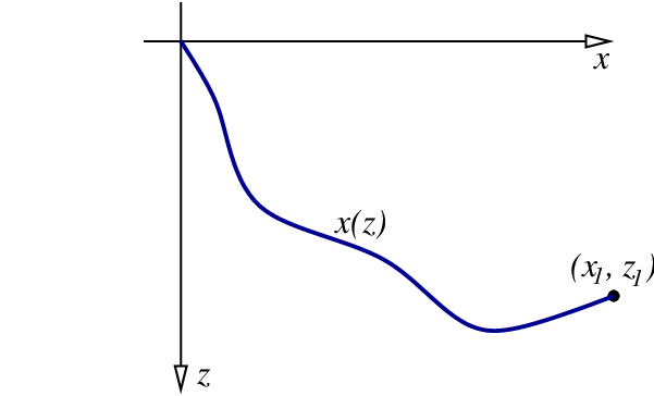
The shape of the slide is specified by the unknown function $x(z)$; this curve in the $x$-$z$ plane is required to link the points $(0,0)$ and $(x_1,z_1)$. The increment of length on the curve is given by
\[ ds = \sqrt{dx^2 + dz^2} = \sqrt{1 + (dx/dz)^2}\, dz = \sqrt{1 + x^{\prime 2}}\, dz, \]
where we now use $x'$ to denote $dx/dz$. The speed of the particle on the slide is $v = ds/dt$, and the increment of time is given by $dt = ds/v$. The total time required by the particle to reach the point $(x_1,z_1)$ is then
\[ t = \int \frac{ds}{v} = \int_0^{z_1} \frac{ \sqrt{1 + x^{\prime 2}} }{v(z)}\, dz. \]
To calculate $v(z)$ we appeal to the conservation of mechanical energy. In this situation the particle moves under the action of gravity, and its total energy is $E = \frac{1}{2} m v^2 - m g z$. It is stated that the particle proceeds from rest ($v=0$) at the upper point of the slide ($z = 0$), and we conclude from this that its total energy is zero. As a consequence we find that $\frac{1}{2} m v^2 = m g z$, or $v(z) = \sqrt{2 g z}$. We therefore have
\[ t = \frac{1}{\sqrt{2 g}} \int_0^{z_1} \frac{ \sqrt{1 + x^{\prime 2}} }{\sqrt{z}}\, dz, \]
and the functional that we wish to minimize is
\begin{equation} \sqrt{2 g} t[x] = \int_0^{z_1} \frac{ \sqrt{1 + x^{\prime 2}} }{\sqrt{z}}\, dz. \tag{2.2.13} \end{equation}
Here the role of the parameter is played by $z$, and the function $G$ is given by
\begin{equation} G(x,x') = \frac{ \sqrt{1 + x^{\prime 2}} }{\sqrt{z}}. \tag{2.2.14} \end{equation}
Notice that this depends only on $x'$; there is no explicit dependence on $x$. Notice further that there is an explicit dependence on the parameter $z$.
The EL equation for this situation is
\[ \frac{\partial G}{\partial x'} = \frac{x'}{\sqrt{z}\sqrt{1 + x^{\prime 2}}}, \]
and the EL equation reduces to
\[ \frac{x'}{\sqrt{z}\sqrt{1 + x^{\prime 2}}} = \frac{1}{\sqrt{2 a}}. \]
This can easily be solved for $x'$, and we obtain
\[ x' = \frac{z}{\sqrt{2 a z - z^2}}. \]
This equation, finally, can be integrated, and a formal solution to our problem is
\begin{equation} x(z) = \int_0^z \frac{z\, dz}{\sqrt{2 a z - z^2}}. \tag{2.2.15} \end{equation}
It is this integral that determines the shape of the minimal slide.
Exercise 2.3: Make sure that you can reproduce the steps that lead to Eq.(2.2.15).
To evaluate the integral of Eq.(2.2.15) we change the variable of integration from $z$ to $\theta$ using the transformation
\[ z = a(1 - \cos\theta), \]
which implies $dz = a\sin\theta\, d\theta$. The angle $\theta$ runs from $0$ when $z = 0$ to $\theta_1$ when $z = z_1$. After a short calculation we find that $2az - z^2 = a^2 \sin^2\theta$, and it follows that
\[ x = a \int_0^\theta (1 - \cos\theta)\, d\theta = a(\theta - \sin\theta). \]
The shape of the slide is therefore described by the parametric equations
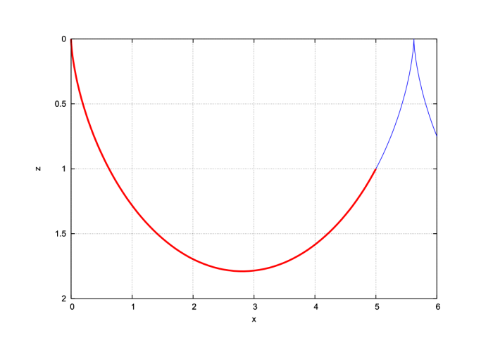
\begin{equation} x(\theta) = a(\theta - \sin\theta), \qquad z(\theta) = a(1 - \cos\theta)\, \qquad 0 \leq \theta \leq \theta_1. \tag{2.2.16} \end{equation}
These describe a curve known as a cycloid. The constants $a$ and $\theta_1$ are determined by the condition that $x = x_1$ and $z = z_1$ when $\theta = \theta_1$. For example, if we choose $x_1 = 5$ and $z_1 = 1$, then we need $a \simeq 0.89483$ and $\theta_1 \simeq 4.5946$. This particular slide is shown in Fig.2.6. The figure reveals that contrary to expectations, the slide does not always go down; it indeed turns around when $\theta = \pi \simeq 3.1416$.
Exercise 2.4: Make sure that you can reproduce the steps that lead to Eq.(2.2.16). Check that the constants $a \simeq 0.89483$ and $\theta_1 \simeq 4.5946$ do indeed produce $x_1 = 5$ and $z_1 = 1$. Can you devise a method to determine $a$ and $\theta_1$ given a choice for $x_1$ and $z_1$?
This feature of the minimal slide is surprising. Can we be sure that this slide truly minimizes the time? Would not a straight slide do a better job? To convince ourselves that we do have the minimal slide, let us compare the times required for the particle to go from $(0,0)$ to $(5,1)$ when it uses either the cycloid or a straight slide. We shall calculate $\sqrt{2 g} t[x]$ for each case and compare the answers.
For the cycloid we have
\[ \sqrt{2 g} t_{\rm cycloid} = \int_0^{z_1} \frac{ \sqrt{1 + x^{\prime 2}} }{\sqrt{z}}\, dz. \]
With the change of variables introduced above we have $x' = (dx/d\theta)/(dz/d\theta) = (1-\cos\theta)/\sin\theta$, so that
\[ \sqrt{1 + x^{\prime 2}} = \frac{\sqrt{\sin^2\theta + (1-\cos\theta)^2}}{\sin\theta} = \frac{\sqrt{2(1-\cos\theta)}}{\sin\theta}. \]
It follows that
\[ \sqrt{2 g} t_{\rm cycloid} = \int_0^{\theta_1} \frac{\sqrt{2(1-\cos\theta)}}{\sin\theta} \frac{a \sin\theta\, d\theta}{\sqrt{a(1-\cos\theta)}} = \sqrt{2a} \int_0^{\theta_1} d\theta, \]
or
\[ \sqrt{2 g} t_{\rm cycloid} = \sqrt{2 a}\theta_1 \simeq 6.1466, \]
using the numerical values listed previously.
The shape of the straight slide is described by $x = 5z$, which implies that $x' = 5$. In this case we have
\[ \sqrt{2 g} t_{\rm straight} = \int_0^1 \frac{\sqrt{26}}{\sqrt{z}}\, dz = 2 \sqrt{26} z^{1/2} \Bigr|^1_0, \]
or
\[ \sqrt{2 g} t_{\rm straight} = 2\sqrt{26} \simeq 10.198, \]
and this is a larger number.
We have found that, sure enough, $t_{\rm cycloid} < t_{\rm straight}$. The particle spends less time on the cycloid than on the straight slide, in spite of the fact that loses speed on the way up toward $(x_1,z_1)$. The reason is that it picks up a lot of speed on the way down, and this more than makes up for the loss of speed on the way up. The straight slide just does not measure up.
2.2.6 Multiple Paths
It is useful, and necessary, to generalize the calculus of variations to functionals $A$ that depend not on one path only, but on a collection of paths. In this final subsection we consider the task of extremizing the multi-path functional
\begin{equation} A[y_1,y_2,\cdots] = \int_{s_0}^{s_1} G(y_1,y'_1;y_2,y'_2;\cdots)\, ds \tag{2.2.17} \end{equation}
with respect to each individual path $y_a(s)$; the index $a = 1, 2, \cdots$ is used to label each path within the collection.
This generalization is straightforward. For each variable $y_a(s)$ within the collection we select a reference path $\bar{y}_a(s)$ and we calculate $A[\bar{y}_1,\bar{y}_2,\cdots]$. We then displace each path from $\bar{y}_a(s)$ to $\bar{y}_a(s) + \delta y_a(s)$ and calculate the new value $A[\bar{y}_1 + \delta y_1, \bar{y}_2 + \delta y_2, \cdots]$ for the functional. The extremum of $A$ is found by demanding that the variation $\delta A = A[\bar{y}_1 + \delta y_1, \bar{y}_2 + \delta y_2, \cdots] - A[\bar{y}_1,\bar{y}_2,\cdots]$ vanish to first order in the displacements $\delta y_a(s)$. As before we impose that the reference and displaced paths all begin and end at the same end points, $y_a(s_0)$ and $y_a(s_1)$. We therefore impose that the variations $\delta y_a$ all vanish at the end points, $\delta y_a(s_0) = 0 = \delta y_a(s_1)$.
The change in functional that occurs when we displace the paths from the reference paths $\bar{y}_a(s)$ is
\[ \delta A = \int_{s_0}^{s_1} \Bigl[ G(\bar{y}_1 + \delta y_1, \bar{y}'_1 + \delta y_1'; \bar{y}_2 + \delta y_2, \bar{y}'_2 + \delta y_2'; \cdots) - G(\bar{y}_1, \bar{y_1}'; \bar{y}_2, \bar{y}_2'; \cdots) \Bigr]\, ds. \]
By Taylor's theorem,
\begin{align} G(\bar{y}_1 + \delta y_1, \bar{y}'_1 + \delta y_1'; \bar{y}_2 + \delta y_2, \bar{y}'_2 + \delta y_2'; \cdots) = G(\bar{y}_1, \bar{y_1}'; \bar{y}_2, \bar{y}_2'; \cdots) \\ + \frac{\partial G}{\partial y_1} \biggr|_{y_1=\bar{y}_1, y_1'=\bar{y}'_1; y_2=\bar{y}_2, y_2'=\bar{y}'_2; \cdots} \delta y_1 + \frac{\partial G}{\partial y_1'} \biggr|_{y_1=\bar{y}_1, y_1'=\bar{y}'_1; y_2=\bar{y}_2, y_2'=\bar{y}'_2; \cdots} \delta y_1' \\ + \frac{\partial G}{\partial y_2} \biggr|_{y_1=\bar{y}_1, y_1'=\bar{y}'_1; y_2=\bar{y}_2, y_2'=\bar{y}'_2; \cdots} \delta y_2 + \frac{\partial G}{\partial y_2'} \biggr|_{y_1=\bar{y}_1, y_1'=\bar{y}'_1; y_2=\bar{y}_2, y_2'=\bar{y}'_2; \cdots} \delta y_2' // + \cdots. \end{align}
Here $G$ is differentiated with respect to each one of its variables, and the partial derivatives are evaluated on the reference paths; we discard all terms that are not linear in the displacements $\delta y_a$ and $\delta y_a'$. We have, in a more compact notation,
\[ \delta A = \int_{s_0}^{s_1} \sum_a \biggl( \frac{\partial G}{\partial y_a} \delta y_a + \frac{\partial G}{\partial y_a'} \delta y_a' \biggr)\, ds, \]
where we sum over all the variables and omit the warning that all partial derivatives must be evaluated on the reference paths, at $y_a = \bar{y}_a$ and $y_a' = \bar{y}_a'$.
We now write
\[ \delta y_a' \equiv y_a' - \bar{y}_a' = \frac{d}{ds} \bigl( y_a - \bar{y}_a \bigr) = \frac{d}{ds} \delta y_a \]
and express the second term within the integral as
\[ \frac{\partial G}{\partial y_a'} d(\delta y_a) = d \biggl( \frac{\partial G}{\partial y_a'} \delta y_a \biggr) - \delta y_a d \biggl( \frac{\partial G}{\partial y_a'} \biggr). \]
Integrating this term by parts gives
\[ \delta A = \sum_a \frac{\partial G}{\partial y_a'} \delta y_a \biggr|^{s_1}_{s_0} + \sum_a \int_{s_0}^{s_1} \biggl( \frac{\partial G}{\partial y_a} - \frac{d}{ds} \frac{\partial G}{\partial y_a'} \biggr) \delta y_a\, ds. \]
Because the displacements must vanish at the end points, the two boundary terms disappear. And because each displacement $\delta y_a(s)$ is independent of any other displacement, and the displacements are arbitrary in the interval $s_0 < s < s_1$, we conclude that
\begin{equation} \delta A = 0 \qquad \Rightarrow \qquad \frac{d}{ds} \frac{\partial G}{\partial y_a'} - \frac{\partial G}{\partial y_a} = 0. \tag{2.2.18} \end{equation}
We have one EL equation for each path $y_a(s)$. This simple statement provides the desired generalization of the calculus of variations to multi-path functionals.
2.3 Hamilton's Principle of Least Action
In Chapter 1 we saw that Newton's law, $\boldsymbol{F} = m \boldsymbol{a}$, can serve as the very foundation of all of mechanics; conservation of momentum, angular momentum, and energy could be derived as a consequence of this dynamical law. In this section we officially replace this old foundation by a new one, which is at once more practical, more powerful, and more easily generalizable to other areas of physics. This new foundation will be Hamilton's principle of least action; the dynamical law $\boldsymbol{F} = m \boldsymbol{a}$, and the statements of conservation, will all be derived as consequences of this new principle.
The principle of least action states that of all the paths $q_a(t)$ that a system of particles could take to go from an initial configuration $q_a(t_0)$ to a final configuration $q_a(t_1)$, the paths $\bar{q}_a(t)$ that the particles actually take are the ones that minimize the action functional
\begin{equation} S[q_a] = \int_{t_0}^{t_1} L(q_a,\dot{q}_a)\, dt, \tag{2.3.1} \end{equation}
where
\begin{equation} L = T - V \tag{2.3.2} \end{equation}
is the Lagrangian function of the mechanical system. The Lagrangian is the difference between $T$, the system's total kinetic energy, and $V$, the total potential energy. The Lagrangian can be expressed in any system of generalized coordinates $q_a$ that conveniently describe the system's degrees of freedom. Because the Lagrangian is a scalar function (as opposed to a vectorial function), the choice of coordinates is immaterial to the formulation of Hamilton's principle. In particular, it is not necessary to adopt Cartesian coordinates attached to an inertial frame. (Of course, nothing prevents us from making this choice if it is convenient.)
To find the paths $\bar{q}_a(t)$ that minimize the action functional we follow the techniques developed in Sec.2.2. Here $S[q_a]$ is a multi-path functional, and the paths $q_a(t)$ play the role of the functions $y_a(s)$; the Lagrangian plays the role of the function $G$, and the parameter is the time $t$. There is no need to repeat the calculations described in Sec.2.2.6; the conclusion is
\begin{equation} \delta S = 0 \qquad \Rightarrow \qquad \frac{d}{dt} \frac{\partial L}{\partial \dot{q}_a} - \frac{\partial L}{\partial q_a} = 0. \tag{2.3.3} \end{equation}
These are the Euler-Lagrange (EL) equations for the mechanical system; there is one EL equation for each degree of freedom. The EL equations, when fully worked out, become a set of second-order differential equations for the paths $q_a(t)$. The solutions to these equations, which much be subjected to the boundary conditions at $t = t_0$ and $t = t_1$, are the paths $\bar{q}_a(t)$ that minimize the action functional.
We have already seen in Sec.2.1 that when the generalized coordinates $q_a(t)$ of a particle are Cartesian, so that the Lagrangian takes the form $L = \frac{1}{2} m (\dot{x}^2 + \dot{y}^2 + \dot{z}^2) - V(x,y,z)$, then the EL equations become the vectorial equation $m \boldsymbol{a} + \boldsymbol{\nabla} V = \boldsymbol{0}$. Recalling that the force acting on the particle is $\boldsymbol{F} = -\boldsymbol{\nabla} V$, this is obviously $\boldsymbol{F} = m \boldsymbol{a}$, and we have derived Newton's fundamental law from a deeper principle, Hamilton's principle of least action. The beauty of this Lagrangian formulation of mechanics, however, is not so much that Newton's equation follows from a deeper principle. Its beauty is much more in the fact that Hamilton's principle frees us from the need to always set up the equations in terms of Cartesian coordinates. Any system of generalized coordinates $q_a(t)$ will do; they all lead to the EL equations of Eq.(2.3.3), and the choice is entirely one of convenience.
In the following sections we will explore the power of Hamilton's principle in a number of applications. We will take full advantage of the generalized nature of the coordinates $q_a(t)$, and the EL equations will allow us to derive the equations of motion very efficiently, with far less effort than would be required in the traditional Newtonian formulation.
2.4 Applications of Lagrangian Mechanics
2.4.1 Equations of Motion in Cylindrical Coordinates
As was just stated, the principal advantage of the Lagrangian formulation of mechanics is that it is based on a scalar function $L$ which can be expressed in any coordinate system whatever. We shall begin our discussion with a derivation of the equations of motion in cylindrical coordinates; the case of spherical coordinates will considered next.
Suppose that a particle moves in the presence of a potential $V$ that is most simply expressed in terms of cylindrical coordinates $(\rho, \phi, z)$. These are related to the usual Cartesian coordinates $(x, y, z)$ by
\begin{equation} x = \rho \cos\phi, \qquad y = \rho \sin\phi, \qquad z = z. \tag{2.4.1} \end{equation}
To use cylindrical coordinates would be advantageous, for example, when the potential is axially symmetric, so that it depends only on $\rho$ and $z$, or cylindrically symmetric, when it depends only on $\rho$.
From Eq.(2.4.1) we obtain the total differentials
\begin{align} dx &= (\cos\phi)\, d\rho - (\rho\sin\phi)\, d\phi, \\ dy &= (\sin\phi)\, d\rho + (\rho\cos\phi)\, d\phi, \\ dz &= dz. \end{align}
It follows that the squared distance between two neighbouring points is given by $ds^2 = dx^2 + dy^2 + dz^2$, or
\begin{equation} ds^2 = d\rho^2 + \rho^2\, d\phi^2 + dz^2. \tag{2.4.2} \end{equation}
The squared velocity is then
\[ v^2 = \Bigl(\frac{ds}{dt} \Bigr)^2 \\ &= \dot{\rho}^2 + \rho^2 \dot{\phi}^2 + \dot{z}^2, \]
and the particle's kinetic energy is $T = \frac{1}{2} m (\dot{\rho}^2 + \rho^2 \dot{\phi}^2 + \dot{z}^2)$. The Lagrangian is therefore
\begin{equation} L(\rho,\dot{\rho};\phi,\dot{\phi};z,\dot{z}) = \frac{1}{2} m (\dot{\rho}^2 + \rho^2 \dot{\phi}^2 + \dot{z}^2) - V(\rho,\phi,z). \tag{2.4.3} \end{equation}
Exercise 2.5: Verify Eq.(2.4.2).
The equations of motion for the particle are obtained by substituting $L$ into the EL equations for $q_a = (\rho,\phi,z)$. We begin with the equation for $\rho$. We have, from Eq.(2.4.3),
\[ \frac{\partial L}{\partial \dot{\rho}} = m \dot{\rho}. \]
This implies
\[ \frac{d}{dt} \frac{\partial L}{\partial \dot{\rho}} = m \ddot{\rho}. \]
We also have
\[ \frac{\partial L}{\partial \rho} = m \rho \dot{\phi}^2 - \frac{\partial V}{\partial \rho}, \]
and the EL equation gives
\begin{equation} m\ddot{\rho} - m \rho \dot{\phi}^2 + \frac{\partial V}{\partial \rho} = 0. \tag{2.4.4} \end{equation}
We continue with the equation for $\phi$. We now have
\[ \frac{\partial L}{\partial \dot{\phi}} = m \rho^2 \dot{\phi}, \]
which implies
\[ \frac{d}{dt} \frac{\partial L}{\partial \dot{\phi}} = m \frac{d}{dt} \Bigl( \rho^2 \dot{\phi} \Bigr). \]
Notice that we choose to leave the total time derivative unevaluated; to evaluate it would require some care, because both $\dot{\phi}$ and $\rho^2$ depend on time in this expression. We also have
\[ \frac{\partial L}{\partial \phi} = -\frac{\partial V}{\partial \phi}, \]
and the EL equation gives
\begin{equation} m \frac{d}{dt} \Bigl( \rho^2 \dot{\phi} \Bigr) + \frac{\partial V}{\partial \phi} = 0. \tag{2.4.5} \end{equation}
We conclude with the equation for $z$. Here the computations are quite easy. We have
\[ \frac{\partial L}{\partial \dot{z}} = m \dot{z}, \]
so that
\[ \frac{d}{dt} \frac{\partial L}{\partial \dot{z}} = m \ddot{z}, \]
and we also have
\[ \frac{\partial L}{\partial z} = - \frac{\partial V}{\partial z}. \]
The EL equation for $z$ is therefore
\begin{equation} m \ddot{z} + \frac{\partial V}{\partial z} = 0. \tag{2.4.6} \end{equation}
The equations of motion (2.4.4)--(2.4.6) could also be derived by resolving Newton's equation $\boldsymbol{F} = m \boldsymbol{a}$ in the vectorial basis $(\boldsymbol{\hat{\rho}},\boldsymbol{\hat{\phi}},\boldsymbol{\hat{z}})$. The results would be identical, but the computations would be much more laborious.
Exercise 2.6: Challenge yourself: Derive Eqs.(2.4.4)--(2.4.6) the hard way, as described in the previous paragraph. Begin by computing the acceleration vector $\boldsymbol{a}$ in terms of the cylindrical coordinates $(\rho,\phi,z)$. Next, find the basis vectors $\boldsymbol{\hat{\rho}}$, $\boldsymbol{\hat{\phi}}$, and $\boldsymbol{\hat{z}}$ using the method outlined in Sec.1.2. Finally, resolve the equation $m \boldsymbol{a} + \boldsymbol{\nabla} V = \boldsymbol{0}$ in this basis, and use the chain rule to calculate $\partial V/\partial \rho$ and $\partial V/\partial \phi$ in terms of $\partial V/\partial x$ and $\partial V/\partial y$. The end result should resemble Eqs.(2.4.4)--(2.4.6). If you are not already, after all this you will be fully convinced of the superiority of the Lagrangian methods!
2.4.2 Equations of Motion in Spherical Coordinates
Suppose now that a particle moves in the presence of a potential $V$ that is most simply expressed in terms of spherical coordinates $(r, \theta, \phi)$. Their relation with the usual Cartesian coordinates $(x, y, z)$ is
\begin{equation} x = r \sin\theta \cos\phi, \qquad y = r \sin\theta \sin\phi, \qquad z = r \cos\theta. \tag{2.4.7} \end{equation}
The use of spherical coordinates would be advantageous, for example, when the potential is axially symmetric, so that it depends only on $r$ and $\theta$, or spherically symmetric, when it depends only on $r$.
From Eq.(2.4.7) we obtain the total differentials
\begin{align} dx &= (\sin\theta \cos\phi)\, dr + (r\cos\theta \cos\phi)\, d\theta - (r \sin\theta \sin\phi)\, d\phi, \\ dy &= (\sin\theta \sin\phi)\, dr + (r\cos\theta \sin\phi)\, d\theta + (r \sin\theta \cos\phi)\, d\phi, \\ dz &= (\cos\theta)\, dr - (r\sin\theta)\, d\theta. \end{align}
It follows that the squared distance between two neighbouring points is given by
\begin{equation} ds^2 = dr^2 + r^2\, d\theta^2 + r^2\sin^2\theta\, d\phi^2. \tag{2.4.8} \end{equation}
The squared velocity is then $v^2 = \dot{r}^2 + r^2 \dot{\theta}^2 + r^2\sin^2\theta\, \dot{\phi}^2$, and the Lagrangian is
\begin{equation} L(r,\dot{r};\theta,\dot{\theta};\phi,\dot{\phi}) = \frac{1}{2} m (\dot{r}^2 + r^2 \dot{\theta}^2 + r^2\sin^2\theta\, \dot{\phi}^2) - V(r,\theta,\phi). \tag{2.4.9} \end{equation}
Exercise 2.7: Verify Eq.(2.4.8).
The equations of motion for the particle are obtained by substituting $L$ into the EL equations for $q_a = (r,\theta,\phi)$. We have, from Eq.(2.4.9),
\[ \frac{\partial L}{\partial \dot{r}} = m \dot{r}, \]
so that
\[ \frac{d}{dt} \frac{\partial L}{\partial \dot{r}} = m \ddot{r}. \]
We also have
\[ \frac{\partial L}{\partial r} = m r ( \dot{\theta}^2 + \sin^2\theta\, \dot{\phi}^2 ) - \frac{\partial V}{\partial r}, \]
and the EL equation for $r$ is
\begin{equation} m\ddot{r} - m r ( \dot{\theta}^2 + \sin^2\theta \dot{\phi}^2 ) + \frac{\partial V}{\partial r} = 0. \tag{2.4.10} \end{equation}
Moving on, we now have
\[ \frac{\partial L}{\partial \dot{\theta}} = m r^2 \dot{\theta}, \]
which implies
\[ \frac{d}{dt} \frac{\partial L}{\partial \dot{\theta}} = m \frac{d}{dt} \Bigl( r^2 \dot{\theta} \Bigr). \]
We also have
\[ \frac{\partial L}{\partial \theta} = m r^2 \sin\theta\cos\theta\, \dot{\phi}^2 - \frac{\partial V}{\partial \theta}, \]
and the EL equation gives
\begin{equation} m \frac{d}{dt} \Bigl( r^2 \dot{\theta} \Bigr) - m r^2 \sin\theta\cos\theta\, \dot{\phi}^2 + \frac{\partial V}{\partial \theta} = 0. \tag{2.4.11} \end{equation}
Finally, we have
\[ \frac{\partial L}{\partial \dot{\phi}} = m r^2\sin^2\theta\, \dot{\phi}, \]
which implies
\[ \frac{d}{dt} \frac{\partial L}{\partial \dot{\phi}} = m \frac{d}{dt} \Bigl( r^2\sin^2\theta\, \dot{\phi} \Bigr). \]
We also have
\[ \frac{\partial L}{\partial \phi} = -\frac{\partial V}{\partial \phi}, \]
and the EL equation gives
\begin{equation} m \frac{d}{dt} \Bigl( r^2\sin^2\theta\, \dot{\phi} \Bigr) + \frac{\partial V}{\partial \phi} = 0. \tag{2.4.12} \end{equation}
The equations of motion (2.4.10)--(2.4.12) could also be derived by resolving Newton's equation $\boldsymbol{F} = m \boldsymbol{a}$ in the vectorial basis $(\boldsymbol{\hat{r}},\boldsymbol{\hat{\theta}},\boldsymbol{\hat{\phi}})$. The results would be identical, but as in the preceding subsection the computations would be much more laborious.
Exercise 2.8: Challenge yourself once again: Derive Eqs.(2.4.10)--(2.4.12) the hard way, as described in the previous paragraph. Or finally cry uncle and pledge allegiance to the Lagrangian way of life!
2.4.3 Motion on the Surface of a Cone
As our first real application of the Lagrangian formalism, we consider a particle that is constrained to move on the surface of a cone, subjected to gravity. As shown in Fig.2.7, the cone has an opening angle of $2\alpha$, and it is placed vertically in the gravitational field. The particle is at a distance $r(t)$ from the cone's apex, and at an angle $\phi(t)$ relative to the $x$ axis. Because the particle is confined to the cone's surface, its angle $\theta$ with respect to the $z$ axis is a constant; it is in fact equal to $\alpha$.
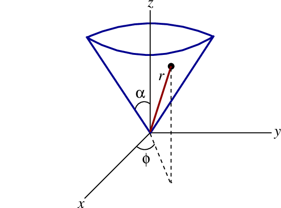
The motion of the particle is best described in terms of spherical coordinates $(r,\theta,\phi)$, with $\theta$ restricted at all times to the value $\alpha$. According to the results of Sec.2.4.2, its kinetic energy is $T = \frac{1}{2} m (\dot{r}^2 + r^2\sin^2\alpha\, \dot{\phi}^2)$, and its potential energy is $V = m g z = mgr\cos\alpha$. The Lagrangian is therefore
\begin{equation} L(r,\dot{r};\phi,\dot{\phi}) = \frac{1}{2} m (\dot{r}^2 + r^2\sin^2\alpha\, \dot{\phi}^2) - m g r \cos\alpha. \tag{2.4.13} \end{equation}
The equations of motion for $r(t)$ and $\phi(t)$ are obtained by substituting this Lagrangian into the EL equations.
We have
\[ \frac{\partial L}{\partial \dot{r}} = m \dot{r}, \]
so that
\[ \frac{d}{dt} \frac{\partial L}{\partial \dot{r}} = m \ddot{r}. \]
We also have
\[ \frac{\partial L}{\partial r} = m r \sin^2\alpha\, \dot{\phi}^2 - mg\cos\alpha, \]
and the EL equation for $r$ is
\begin{equation} \ddot{r} - r \sin^2\alpha\, \dot{\phi}^2 + g\cos\alpha = 0. \tag{2.4.14} \end{equation}
Moving on, we observe that $L$ is independent of $\phi$, and the fact that $\partial L/\partial \phi = 0$ means that the EL equation for $\phi$ reduces to
\[ \frac{d}{dt} \frac{\partial L}{\partial \dot{\phi}} = 0. \]
This implies that the quantity $\partial L/\partial \dot{\phi}$ is a constant, which we shall call $m h$. Calculating the partial derivative gives $\partial L/\partial \dot{\phi} = m r^2\sin^2\alpha\, \dot{\phi}$, and we finally obtain the statement
\begin{equation} r^2 \sin^2\alpha\, \dot{\phi} = h = \text{constant}. \tag{2.4.15} \end{equation}
The quantity $h$ is readily interpreted as the $z$ component of the particle's reduced angular momentum vector, and it is a constant of the motion. Equation (2.4.15) shows that $\dot{\phi}$ is always of the same sign; the angular part of the motion is monotonic.
Substituting $\dot{\phi} = h/(r^2\sin^2\alpha)$ into Eq.(2.4.14) produces
\[ \ddot{r} - \frac{h^2}{r^3\sin^2\alpha} + g\cos\alpha = 0. \]
This equation can be integrated by using the standard trick of multiplying each term by $\dot{r}$ (recall that we used this trick back in Sec.1.5.6). We have
\[ \ddot{r}\dot{r} - \frac{h^2 \dot{r}}{r^3\sin^2\alpha} + g \dot{r} \cos\alpha = 0, \]
or
\[ \frac{d}{dt} \biggl( \frac{1}{2} \dot{r}^2 + \frac{h^2}{2r^2\sin^2\alpha} + gr\cos\alpha \biggr) = 0. \]
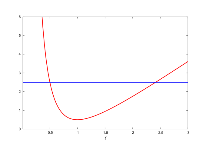
This finally gives us the conservation statement
\begin{equation} \frac{1}{2} \dot{r}^2 + \nu(r) = \varepsilon = \text{constant}, \tag{2.4.16} \end{equation}
where $\varepsilon$ is the particle's reduced total mechanical energy, and
\begin{equation} \nu(r) = \frac{h^2}{2r^2\sin^2\alpha} + gr\cos\alpha \tag{2.4.17} \end{equation}
is an effective potential for the radial part of the motion. Equations (2.4.16) and (2.4.17) give rise to the energy diagram of Fig.2.8. From this diagram we immediately conclude that the motion takes place between two turning points at $r = r_\pm$; these are determined by the condition $\nu(r_\pm) = \varepsilon$.
To obtain a full picture of the motion Eqs.(2.4.14) and (2.4.15) must be integrated numerically. Results of such a numerical integration are presented in Fig.2.9. To carry out these integrations the equations are recast into the following set of first-order equations:
\[ \dot{r} = v, \qquad \dot{v} = \frac{h^2}{r^3\sin\alpha} - g\cos\alpha, \qquad \dot{\phi} = \frac{h}{r^2\sin^2\alpha}, \]
where we have introduced the auxiliary variable $v$. We start the integration at $r=r_-$, setting $v=0$ (as we must) and $\phi = 0$. The constant $h$ can be determined in terms of $r_-$ and $r_+$ by using the relation $\nu(r_-) = \nu(r_+)$, which follows from Eq.(2.4.16). The result is
\[ h^2 = 2 g \sin^2\alpha \cos\alpha \frac{(r_+ r_-)^2}{r_+ + r_-}. \]
Exercise 2.9: Verify the quoted relation between $h^2$ and $r_\pm$.
2.4.4 Spherical Pendulum
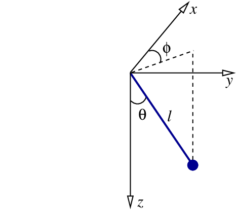
We now examine the situation of a pendulum which is free to move in all directions about its pivot point. The pendulum has a mass $m$, a constant length $\ell$, and its motion is described in terms of the two angles $\theta(t)$ and $\phi(t)$, as shown in Fig.2.10. These coordinates are related to the standard Cartesian coordinates by
\[ x = \ell \sin\theta \cos\phi, \qquad y = \ell \sin\theta \sin\phi, \qquad z = \ell \cos\theta. \]
As shown in the figure, the $z$ axis is pointing down, in the direction of the gravitational acceleration $\boldsymbol{g}$. It is clear that we are once more dealing with spherical coordinates. This time, however, it is the radial coordinate $r$ that is held fixed to the value $\ell$. According to the results of Sec.2.4.2 the pendulum's kinetic energy is $T = \frac{1}{2} m \ell^2 (\dot{\theta}^2 + \sin^2\theta\, \dot{\phi}^2)$. Its potential energy is $V = -m g z = -m g \ell \cos\theta = -m\ell^2 \omega^2\cos\theta$, where we have re-introduced the quantity
\begin{equation} \omega = \sqrt{g/\ell}. \tag{2.4.18} \end{equation}
The pendulum's Lagrangian is
\begin{equation} L(\theta,\dot{\theta};\phi,\dot{\phi}) = \frac{1}{2} m \ell^2 (\dot{\theta}^2 + \sin^2\theta\, \dot{\phi}^2) + m\ell^2 \omega^2 \cos\theta. \tag{2.4.19} \end{equation}
The equations of motion for $\theta(t)$ and $\phi(t)$ are obtained by substituting this Lagrangian into the EL equations.
We compute
\[ \frac{\partial L}{\partial \dot{\theta}} = m \ell^2 \dot{\theta}, \]
which implies
\[ \frac{d}{dt} \frac{\partial L}{\partial \dot{\theta}} = m \ell^2 \ddot{\theta}. \]
We also have
\[ \frac{\partial L}{\partial \theta} = m \ell^2 \sin\theta \cos\theta\, \dot{\phi}^2 - m\ell^2 \omega^2 \sin\theta, \]
and the EL equation for $\theta$ is
\begin{equation} \ddot{\theta} - \sin\theta \cos\theta\, \dot{\phi}^2 + \omega^2 \sin\theta = 0. \tag{2.4.20} \end{equation}
Moving on, we observe that $L$ is independent of $\phi$, and the fact that $\partial L/\partial \phi = 0$ means that the EL equation for $\phi$ reduces to
\[ \frac{d}{dt} \frac{\partial L}{\partial \dot{\phi}} = 0. \]
This implies that the quantity $\partial L/\partial \dot{\phi}$ is a constant, which we shall call $m \ell^2 h$. Calculating the partial derivative gives $\partial L/\partial \dot{\phi} = m \ell^2\sin^2\theta\, \dot{\phi}$, and we finally obtain the statement
\begin{equation} \sin^2\theta\, \dot{\phi} = h = \text{constant}. \tag{2.4.21} \end{equation}
The quantity $h$ is once more interpreted as the $z$ component of the pendulum's reduced angular momentum vector, and it is a constant of the motion. In the special case $h=0$ the pendulum is prevented to move in the $\phi$ direction, and Eq.(2.4.20) for $\theta$ reduces to $\ddot{\theta} + \omega^2 \sin\theta = 0$; this is the same equation that was first derived in Sec.1.3.7, and then again in Sec.2.1, and which describes the motion of a planar pendulum. In the general case ($h \neq 0$) we see that $\dot{\phi}$ is always of the same sign, so that $\phi(t)$ is a monotonic function of time; this means that the pendulum rotates in a consistent direction around the $z$ axis.
With the substitution $\dot{\phi} = h/\sin^2\theta$ Eq.(2.4.20) becomes
\[ \ddot{\theta} - \frac{h^2 \cos\theta}{\sin^3\theta} + \omega^2\sin\theta = 0. \]
Multiplying each term by $\dot{\theta}$ allows us to integrate this equation. The result is the conservation statement
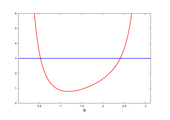
\begin{equation} \frac{1}{2} \dot{\theta}^2 + \nu(\theta) = \varepsilon = \text{constant}, \tag{2.4.22} \end{equation}
where $\varepsilon$ is the pendulum's reduced total mechanical energy, and
\begin{equation} \nu(\theta) = \frac{h^2}{2\sin^2\theta} - \omega^2\cos\theta \tag{2.4.23} \end{equation}
is an effective potential for the motion in the $\theta$ direction. Equations (2.4.22) and (2.4.23) give rise to the energy diagram of Fig.2.11. From this diagram we may immediately conclude that the motion takes place between two turning points at $\theta = \theta_\pm$; these are determined by the condition $\nu(\theta_\pm) = \varepsilon$.
Exercise 2.10: Verify that Eqs.(2.4.22) and (2.4.23) do indeed follow from the equations of motion.
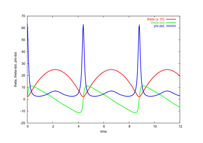
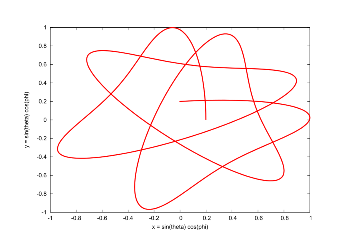
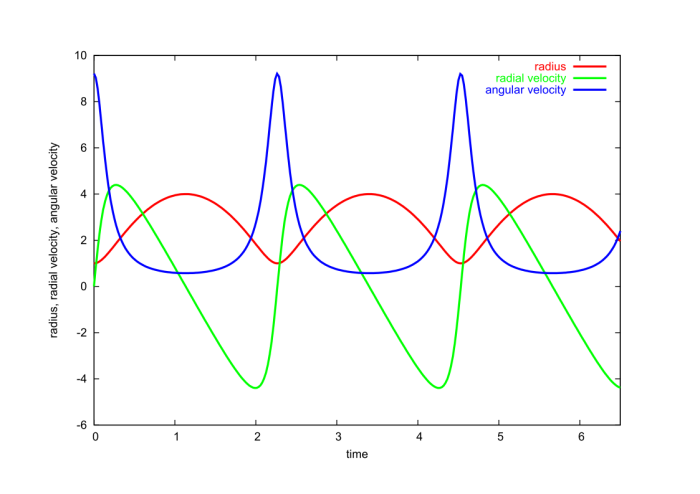
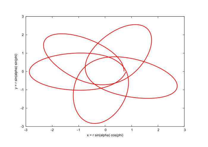
In Fig.2.12 we present the results of a numerical integration of the equations of motion, which we recast into the first-order form
\[ \dot{\theta} = v, \qquad \dot{v} = \frac{h^2 \cos\theta}{\sin^3\theta} - \omega^2\sin\theta, \qquad \dot{\phi} = \frac{h}{\sin^2\theta}. \]
We start the integration at $\theta =\theta_-$, setting $v=0$ and $\phi = 0$. The constant $h$ can be determined in terms of $\theta_-$ and $\theta_+$ by using the relation $\nu(\theta_-) = \nu(\theta_+)$, which follows from Eq.(2.4.22). The result, after some algebra, is
\[ h^2 = 2 \omega^2 \frac{(\sin\theta_+ \sin\theta_-)^2 (\cos\theta_- - \cos\theta_+)}{(\sin\theta_+ - \sin\theta_-) (\sin\theta_+ + \sin\theta_-)}. \]
Exercise 2.11: Verify the quoted relation between $h^2$ and $\theta_\pm$.
2.4.5 Rotating Pendulum
Another variation on the pendulum theme has the pivot point of a planar pendulum forced to rotate with a constant angular velocity $\Omega$ on a circle of radius $a$. This situation is shown in Fig.2.13. Once more we describe the motion of the pendulum in terms of the swing angle $\theta(t)$, which is defined relative to the vertical direction; this we now associate with the $y$-direction.
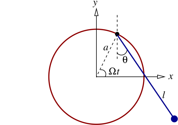
Figure 2.13: The motion of a rotating pendulum is described in terms of the swing angle $\theta(t)$. The pivot point rotates with a constant angular velocity $\Omega$ on a circle of radius $a$.
The Cartesian coordinates of the pendulum, relative to the pivot point, are
\[ x_{\rm relative} = \ell \sin\theta, \qquad y_{\rm relative} = -\ell \cos\theta. \]
The Cartesian coordinates of the pivot point are
\[ x_{\rm pivot} = a \cos\Omega t, \qquad y_{\rm pivot} = a \sin\Omega t. \]
The Cartesian coordinates of the pendulum, relative to the origin of the coordinate system, are therefore
\begin{equation} x = a\cos\Omega t + \ell \sin\theta, \qquad y = a\sin\Omega t - \ell \cos\theta. \tag{2.4.24} \end{equation}
The components of the velocity vector are
\[ \dot{x} = -a\Omega \sin\Omega t + \ell \dot{\theta} \cos\theta, \qquad \dot{y} = a\Omega \cos\Omega t + \ell \dot{\theta} \sin\theta. \]
The squared velocity is then calculated as
\[ v^2 = \dot{x}^2 + \dot{y}^2 = (a\Omega)^2 + 2 a \ell \Omega \dot{\theta} \sin(\theta - \Omega t) + \ell^2 \dot{\theta}^2, \]
and the kinetic energy of the pendulum is $T = \frac{1}{2} m v^2$. Its potential energy is $V = mgy = mg(a \sin\Omega t - \ell \cos\theta)$.
Exercise 2.12: Verify the preceding result for $v^2$.
The Lagrangian of the rotating pendulum is, finally,
\begin{equation} L(\theta,\dot{\theta};t) = \frac{1}{2} m \Bigl[ (a\Omega)^2 + 2 a \ell \Omega \dot{\theta} \sin(\theta - \Omega t) + \ell^2 \dot{\theta}^2 \Bigr] - m \ell \omega^2 (a \sin\Omega t - \ell \cos\theta), \tag{2.4.25} \end{equation}
where we have once more introduced $\omega^2 = g/\ell$. A new feature of this Lagrangian is that it depends explicitly on time; this comes about because the pendulum is not left alone to its own devices, but is instead acted upon and forced to follow a rotational motion. In this circumstance we cannot expect the energy of the pendulum to be conserved: There will be at all times a transfer of energy between the pendulum and the external agent that is responsible for the rotational motion. Globally the total energy is conserved, but the energy of the pendulum is not individually conserved.
To obtain the equation for motion we must first calculate
\[ \frac{\partial L}{\partial \dot{\theta}} = m a \ell \Omega \sin(\theta-\Omega t) + m \ell^2 \dot{\theta}. \]
Differentiating this with respect to time gives
\[ \frac{d}{dt} \frac{\partial L}{\partial \dot{\theta}} = m a \ell \Omega \cos(\theta-\Omega t)(\dot{\theta} - \Omega) + m \ell^2 \ddot{\theta}. \]
We next compute
\[ \frac{\partial L}{\partial \theta} = m a \ell \Omega \dot{\theta} \cos(\theta - \Omega t) - m\ell^2 \omega^2 \sin\theta, \]
and substituting all this into the EL equation produces
\begin{equation} \ddot{\theta} + \omega^2 \sin\theta - (a/\ell) \Omega^2 \cos(\theta - \Omega t) = 0. \tag{2.4.26} \end{equation}
This is the equation of motion of a rotating pendulum.
Equation (2.4.26) cannot be integrated with the help of the $\dot{\theta}$ trick; this is prevented by the fact that the equation depends explicitly on time through the term in $\cos(\theta-\Omega t)$. As a consequence, the motion cannot be analyzed with the help of an energy diagram; this can be understood from the very fact that the total mechanical energy of the rotating pendulum is not conserved. The only tool that remains at our disposal to analyze the motion is numerical integration, and Fig.2.14 displays the results.
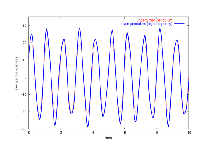
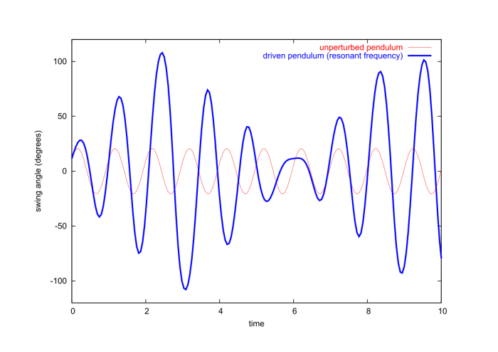
The graphs reveal that when the pendulum is driven at a frequency $\Omega$ that is close to its natural frequency $\omega$, the response is more violent: the amplitude of the oscillations is then much larger. This is the phenomenon of resonance. This phenomenon can be illustrated in the context of a simpler model, one which can be solved exactly. We consider a simple harmonic oscillator which is driven by an oscillating external force. The equations of motion for this simplified model is
\begin{equation} \ddot{\theta} + \omega^2 \theta = A \cos\Omega t. \tag{2.4.27} \end{equation}
When $\Omega \neq \omega$ a solution to this equation is
\begin{equation} \theta(t) = \frac{A}{\omega^2-\Omega^2} \cos\Omega t \qquad (\Omega \neq \omega). \tag{2.4.28} \end{equation}
In this situation the pendulum oscillates at the driving frequency $\Omega$, and the oscillations have a constant amplitude. Notice, however, that the amplitude grows as $\Omega$ approaches the natural frequency $\omega$. The solution of Eq.(2.4.28) is not valid when $\Omega = \omega$. In this case we have instead
\begin{equation} \theta(t) = \frac{At}{2\omega} \sin\omega t \qquad (\Omega = \omega). \tag{2.4.29} \end{equation}
In this case the oscillations keep growing in amplitude; the simple harmonic oscillator is in resonance with the driving force.
Exercise 2.13: Verify that Eqs.(2.4.28) and (2.4.29) are solutions to Eq.(2.4.27). A more challenging question: What is the {\it general solution} to Eq.(2.4.27) when $\Omega \neq \omega$ and when $\Omega = \omega$? The general solution should be parameterized in terms of the initial angle $\theta(0)$ and the initial angular velocity $\dot{\theta}(0)$. What choices of initial conditions give rise to Eqs.(2.4.28) and (2.4.29)?
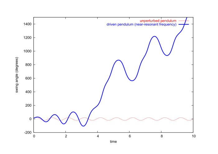
When the rotating pendulum is driven at resonance we observe a growth in the amplitude of oscillations, but this growth is bounded; it saturates and the amplitude then starts to decrease. This saturation is produced by nonlinear effects: When the amplitude grows the natural period of the oscillations changes (as we learned back in Sec.1.3.7) and the pendulum is no longer driven at its natural frequency. As resonance stops the amplitude starts to decrease and the pendulum's natural frequency returns to its original value. At this stage the conditions are once more suitable for a resonant growth of the amplitude, and the cycle repeats.
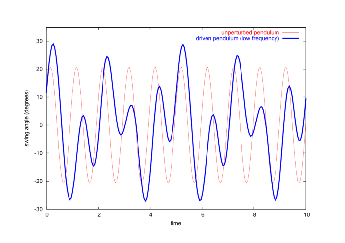
For certain choices of parameters the driving force can have a dramatic influence on the pendulum. This is illustrated in Fig.2.15, for which the driving frequency was set to $\Omega = 0.9 \omega$. Here we see the driving force causing the pendulum to go beyond $\theta = \pi$, completing one or two revolutions before returning to a short oscillation cycle.
2.4.6 Rolling Disk
As our next application we consider a disk of mass $m$ and radius $R$ that rolls without slipping on an inclined plane of total length $\ell$; the plane's inclination relative to the horizontal is $\alpha$. As shown in Fig.2.16, the distance from the top position on the plane to the disk's centre of mass --- its geometric centre --- is denoted $s$, and $\theta$ is the angle of a selected point on the disk's rim relative to an axis perpendicular to the inclined plane
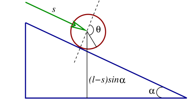
There is both a translational motion of the centre of mass and a rotational motion of the disk in this problem. The disk's kinetic energy is
\[ T = \frac{1}{2} m \dot{s}^2 + \frac{1}{2} I \dot{\theta}^2, \]
where $I = \frac{1}{2} m R^2$ is the disk's moment of inertia. The coordinates $s$ and $\theta$, however, are not independent; they are related by the no-slip condition, which implies $s = R\theta$. So we have $\dot{s} = R\dot{\theta}$ and the kinetic energy becomes
\[ T = \frac{1}{2} m R^2 \dot{\theta}^2 + \frac{1}{4} m R^2 \dot{\theta}^2 = \frac{3}{4} m R^2 \dot{\theta}^2. \]
The disk's potential energy is $V = mgz = mg(l-s)\sin\alpha = mg(\ell - R\theta) \sin\alpha$.
The Lagrangian is therefore
\begin{equation} L(\theta,\dot{\theta}) = \frac{3}{4} m R^2 \dot{\theta}^2 - m g (\ell -R\theta) \sin\alpha. \tag{2.4.30} \end{equation}
To obtain the disk's equation of motion we substitute this into the EL equation. We first compute
\[ \frac{\partial L}{\partial \dot{\theta}} = \frac{3}{2} m R^2 \dot{\theta}, \]
which implies
\[ \frac{d}{dt} \frac{\partial L}{\partial \dot{\theta}} = \frac{3}{2} m R^2 \ddot{\theta}. \]
We also compute
\[ \frac{\partial L}{\partial \theta} = mgR\sin\alpha. \]
The equation of motion is then
\begin{equation} \ddot{\theta} = \frac{2 g \sin\alpha}{3R}, \label{2.4.31} \end{equation}
and we find that the disk is under constant angular acceleration.
If we assume that the disk started with zero angular velocity, then Eq.(2.4.31) integrates to
\begin{equation} \theta(t) = \frac{g\sin\alpha}{3R} t^2. \tag{2.4.32} \end{equation}
The time $t_{\rm bottom}$ required for the disk to reach the bottom of the inclined plane is determined by the condition $\theta(t_{\rm bottom}) = \ell/R$. Solving this gives
\begin{equation} t_{\rm bottom} = \sqrt{ \frac{3\ell}{g\sin\alpha} }. \tag{2.4.33} \end{equation}
Notice that $t_{\rm bottom}$ is independent of $R$, the disk's radius.
2.4.7 Kepler's Problem Revisited
As a final application of the Lagrangian formalism we will rederive the main equations of Kepler's problem. As we shall see, the Lagrangian methods give a much more efficient way of obtaining these equations.
As in Sec.1.5.2 we express the position vectors $\boldsymbol{r}_1$ and $\boldsymbol{r}_2$ of the two massive bodies in terms of the relative separation vector $\boldsymbol{r} = \boldsymbol{r}_1 - \boldsymbol{r}_2$ and the position $\boldsymbol{R}$ of the centre of mass, which is determined by $M \boldsymbol{R} = m_1 \boldsymbol{r}_1 + m_2 \boldsymbol{r}_2$, where $M = m_1 + m_2$ is the total mass. We have $\boldsymbol{r}_1 = \boldsymbol{R} + (m_2/M) \boldsymbol{r}$, $\boldsymbol{r}_2 = \boldsymbol{R} - (m_1/M) \boldsymbol{r}$, and after some algebra we find that the system's kinetic energy is
\begin{align} T &= \frac{1}{2} m_1 \boldsymbol{\dot{r}}_1 \cdot \boldsymbol{\dot{r}}_1 + \frac{1}{2} m_2 \boldsymbol{\dot{r}}_2 \cdot \boldsymbol{\dot{r}}_2 \\ &= \frac{1}{2} M \boldsymbol{\dot{R}} \cdot \boldsymbol{\dot{R}} + \frac{1}{2} \frac{m_1 m_2}{M} \boldsymbol{\dot{r}} \cdot \boldsymbol{\dot{r}}. \end{align}
The system's potential energy, on the other hand, was calculated in Sec.1.5.1, and it is given by
\[ V = -\frac{G m_1 m_2}{r}, \]
where $r = |\boldsymbol{r}| = |\boldsymbol{r}_1 - \boldsymbol{r}_2|$ is the distance between the two bodies. The system's Lagrangian is
\begin{equation} L(\boldsymbol{R},\boldsymbol{\dot{R}};\boldsymbol{r},\boldsymbol{\dot{r}}) = \frac{1}{2} M \boldsymbol{\dot{R}} \cdot \boldsymbol{\dot{R}} + \frac{1}{2} \mu \boldsymbol{\dot{r}} \cdot \boldsymbol{\dot{r}} + \frac{G \mu M}{r}, \tag{2.4.34} \end{equation}
where
\begin{equation} \mu = \frac{m_1 m_2}{M}, \qquad M = m_1 + m_2 \tag{2.4.35} \end{equation}
is known as the reduced mass of the two-body system.
Exercise 2.14: Go through the algebra that leads to our previous expression for the kinetic energy in terms of $\boldsymbol{\dot{R}}$ and $\boldsymbol{\dot{r}}$.
Notice that the Lagrangian of Eq.(2.4.34) separates into two independent pieces. The first piece depends on $\boldsymbol{R}$ only, and is independent of $\boldsymbol{r}$; this is the Lagrangian of the centre of mass,
\[ L_{\rm CM}(\boldsymbol{R},\boldsymbol{\dot{R}}) = \frac{1}{2} M \boldsymbol{\dot{R}} \cdot \boldsymbol{\dot{R}}. \]
The second piece depends on $\boldsymbol{r}$ only, and is independent of $\boldsymbol{R}$; this is the Lagrangian of the relative separation between the two bodies,
\[ L_{\rm rel}(\boldsymbol{r},\boldsymbol{\dot{r}}) = \frac{1}{2} \mu \boldsymbol{\dot{r}} \cdot \boldsymbol{\dot{r}} + \frac{G \mu M}{r}. \]
Notice now that $L_{\rm CM}$ contains only a kinetic-energy term. The absence of a potential-energy term implies that the motion of the centre of mass is free. As a quick calculation will verify, the EL equations for $\boldsymbol{R}$ take the form $\boldsymbol{\ddot{R}} = \boldsymbol{0}$, for which the solution is $\boldsymbol{R}(t) = \boldsymbol{R}(0) + \boldsymbol{\dot{R}}(0) t$. As we have seen in Sec.1.5.2, the centre of mass moves freely, and it can be placed at the origin of an inertial frame. The relative Lagrangian, on the other hand, contains both a kinetic-energy term and a potential-energy term. It describes the motion of a fictitious particle of mass $\mu$ in the gravitational field of a central mass $M$, also fictitious. As we have witnessed before in Sec.1.5.2, our original two-body problem has simplified into an effective one-body problem.
To proceed we may switch from the Cartesian coordinates $\boldsymbol{r} = (x,y,z)$ to any system of generalized coordinates $q_a$. Recalling from Sec.1.5.3 that the motion takes place in the $x$-$y$ plane (a fact that could be re-derived on the basis of Lagrangian mechanics), we adopt the polar coordinates $(r,\phi)$, related to $x$ and $y$ by $x = r\cos\phi$ and $y = r\sin\phi$. We have $\dot{x} = \dot{r} \cos\phi - r\dot{\phi} \sin\phi$, $\dot{y} = \dot{r} \sin\phi + r\dot{\phi} \cos\phi$, and it follows that
\[ \boldsymbol{\dot{r}} \cdot \boldsymbol{\dot{r}} = \dot{x}^2 + \dot{y}^2 = \dot{r}^2 + (r \dot{\phi})^2. \]
The Lagrangian therefore becomes
\begin{equation} L_{\rm rel}(r,\dot{r};\phi,\dot{\phi}) = \frac{1}{2} \mu \Bigl[ \dot{r}^2 + (r \dot{\phi})^2 \Bigr] + \frac{G\mu M}{r}. \tag{2.4.36} \end{equation}
Notice that this Lagrangian is actually independent of $\phi$, a feature that was encountered also in previous examples.
To obtain the equation of motion for $r$ we compute
\[ \frac{\partial L_{\rm rel}}{\partial \dot{r}} = \mu \dot{r} \qquad \Rightarrow \qquad \frac{d}{dt} \frac{\partial L_{\rm rel}}{\partial \dot{r}} = \mu \ddot{r} \]
and
\[ \frac{\partial L_{\rm rel}}{\partial r} = \mu r \dot{\phi}^2 - \frac{G \mu M}{r^2}. \]
This gives
\begin{equation} \ddot{r} - r \dot{\phi}^2 + \frac{G M}{r^2} = 0. \tag{2.4.37} \end{equation}
This is the same statement as Eq.(1.5.25). To obtain the equation of motion for $\phi$ we observe that since $L_{\rm rel}$ is independent of $\phi$, we must have that $\partial L_{\rm rel}/\partial \dot{\phi}$ is a constant of the motion. Calling this constant $\mu h$ and calculating the partial derivative, we get
\begin{equation} r^2 \dot{\phi} = h = \text{constant}. \tag{2.4.38} \end{equation}
This is the same statement as Eq.(1.5.27), and $h$ is identified as the reduced angular momentum of the two-body system.
The equations of motion (2.4.37) and (2.4.38) can be analyzed with the same mathematical techniques as those employed in Sec.1.5. It should be clear that compared with the Newtonian methods of Chapter 1, the Lagrangian methods provide a much simpler way of obtaining these equations.
2.5 Generalized Momenta and Conservation Statements
2.5.1 Conservation of Generalized Momentum
In the applications of Lagrangian mechanics presented in Sec.2.4 it occurred a number of times that the Lagrangian was independent of one of the generalized coordinates (mostly it was the $\phi$ coordinate), and we saw that this fact always translated into the existence of a constant of the motion (which we usually called $h$). A specific example is the case of a particle moving on the surface of a cone (Sec.2.4.3), for which the Lagrangian is indeed independent of $\phi$ and for which the constant of the motion was $h = r^2\sin^2\alpha\, \dot{\phi}$. A similar situation occurred for the spherical pendulum (Sec.2.4.4) and for Kepler's problem (Sec.2.4.7).
It is easy to generalize this discussion and to derive the very useful fact that whenever the Lagrangian does not depend explicitly on one (or more) of the generalized coordinates $q_a$, there exists a corresponding constant of the motion. To establish this statement we shall first introduce the notion of a generalized momentum.
Consider a Lagrangian $L(q_a,\dot{q}_a)$ that depends on a number of generalized coordinates $q_a$ and a number of generalized velocities $\dot{q}_a$. The quantities
\begin{equation} p_a = \frac{\partial L}{\partial \dot{q}_a} \tag{2.5.1} \end{equation}
feature prominently in the EL equations, which can be written in the form
\begin{equation} \dot{p}_a = \frac{\partial L}{\partial q_a}. \tag{2.5.2} \end{equation}
The quantities $p_a$ are the generalized momenta of the mechanical system. There is one generalized momentum $p_a$ for each generalized coordinate $q_a$.
The generalized momenta can represent either a component of the linear-momentum vector or a component of the angular-momentum vector. Generally speaking, whenever $q_a$ represents a linear variable the corresponding $p_a$ will be a linear momentum; and whenever $q_a$ represents an angular variable its corresponding $p_a$ will be an angular momentum. Consider, for example, the Lagrangian of a free particle in cylindrical coordinates (Sec.2.4.1). This is
\[ L = \frac{1}{2} m (\dot{\rho}^2 + \rho^2 \dot{\phi}^2 + \dot{z}^2). \]
The generalized momenta are
\begin{align} p_\rho &= \frac{\partial L}{\partial \dot{\rho}} = m \dot{\rho}, \\ p_\phi &= \frac{\partial L}{\partial \dot{\phi}} = m \rho^2 \dot{\phi}, \\ p_z &= \frac{\partial L}{\partial \dot{z}} = m \dot{z}. \end{align}
In the case of $p_\rho$ and $p_z$ we clearly have quantities that represent components of a linear-momentum vector. But the case of $p_\phi$ is different. Here we have $p_\phi = m(\rho)(\rho \dot{\phi})$, and this clearly represents the component of an angular-momentum vector.
Exercise 2.15: Show that $p_\rho = \boldsymbol{p} \cdot \boldsymbol{\hat{\rho}}$ and $p_z = \boldsymbol{p} \cdot \boldsymbol{\hat{z}}$, where $\boldsymbol{p}$ is the particle's momentum vector. Show, on the other hand, that $p_\phi = \boldsymbol{L} \cdot \boldsymbol{\hat{z}}$, where $\boldsymbol{L}$ is the particle's angular-momentum vector.
Suppose now that a Lagrangian $L(q_1,\dot{q}_1;q_2,\dot{q}_2,\cdots)$ happens not to depend explicitly on one of its generalized coordinates, say $q_*$. Then
\[ \frac{\partial L}{\partial q_*} = 0 \]
and it follows from the EL equation for $q_*$ that
\[ \frac{d p_*}{dt} = 0, \]
where $p_* = \partial L/\partial \dot{q}_*$ is the generalized momentum associated with the coordinate $q_*$. This equation states that $p_*$ is a constant of the motion, and we have established the following theorem:
Whenever the Lagrangian of a mechanical system does not depend explicitly on a generalized coordinate $q_*$, the corresponding generalized momentum $p_* = \partial L/\partial \dot{q}_*$ is a constant of the motion.
A coordinate $q_*$ that does not appear in $L$ is sometimes called a cyclic coordinate. A Lagrangian may contain any number of cyclic coordinates.
As an example consider the following Lagrangian, again in cylindrical coordinates,
\[ L = \frac{1}{2} m ( \dot{\rho}^2 + \rho^2 \dot{\phi}^2 + \dot{z}^2 ) - V(\rho). \]
Here it is assumed that the potential energy $V$ depends only on $\rho$; the mechanical system is cylindrically symmetric. This implies that $\phi$ and $z$ are cyclic coordinates, and that $p_\phi = m\rho^2 \dot{\phi}$ and $p_z = m \dot{z}$ are constants of the motion.
This theorem on cyclic coordinates and conserved quantities is extremely important and very useful. To find all the constants of the motion is usually a key step during the integration of the equations of motion, and the theorem provides a very efficient algorithm to identify at least some of them.
2.5.2 Conservation of Energy
Conservation of total mechanical energy $E$ is also an important aspect of the motion of a mechanical system and a key to solving the equations of motion. In this subsection we show that energy is conserved whenever the Lagrangian does not depend explicitly on time $t$.
To begin the discussion let us consider a Lagrangian $L(q_a,\dot{q}_a,t)$ that depends on a number of generalized coordinates $q_a$, a number of generalized velocities $\dot{q}_a$, and let us consider the possibility that it depends also explicitly on time. (An example is the Lagrangian of a rotating pendulum, which was written down in Sec.2.4.5.) Applying the chain rule, we find that the total time derivative of the Lagrangian is given by
\[ \frac{dL}{dt} = \sum_a \frac{\partial L}{\partial q_a}\, \dot{q}_a + \sum_a \frac{\partial L}{\partial \dot{q}_a}\, \ddot{q}_a + \frac{\partial L}{\partial t}. \]
The first term accounts for the time dependence contained in each $q_a(t)$, the second term for the time dependence contained in each $\dot{q}_a(t)$, and the third term accounts for the explicit dependence of the Lagrangian on $t$.
We have defined the generalized momenta $p_a$ by
\[ p_a = \frac{\partial L}{\partial \dot{q}_a} \]
and the EL equations can be expressed in the form
\[ \dot{p}_a = \frac{\partial L}{\partial q_a}. \]
We make these substitutions in the previous equation, and obtain
\[ \frac{dL}{dt} = \sum_a \Bigl( \dot{p}_a \dot{q}_a + p_a \ddot{q}_a \Bigr) + \frac{\partial L}{\partial t}, \]
or
\[ \frac{dL}{dt} = \frac{d}{dt} \biggl( \sum_a p_a \dot{q}_a \biggr) + \frac{\partial L}{\partial t}, \]
which is equivalent to the previous form by virtue of the chain rule.
We have obtained the equation
\begin{equation} \frac{d}{dt} \biggl( \sum_a p_a \dot{q}_a - L \biggr) = - \frac{\partial L}{\partial t}, \tag{2.5.3} \end{equation}
and a statement of conservation follows immediately:
Whenever $L$ does not depend explicitly on time, so that $\partial L/\partial t = 0$, we have that
\begin{equation} h(q_a,\dot{q}_a) \equiv \sum_a p_a \dot{q}_a - L \tag{2.5.4} \end{equation}
is a constant of the motion, $dh/dt = 0$.
Surely the function $h(q_a,\dot{q}_a)$ must have something to do with the system's total mechanical energy. Let us first figure out the relationship in the context of a simple example. We go back to the Lagrangian of a particle expressed in cylindrical coordinates,
\[ L = \frac{1}{2} m ( \dot{\rho}^2 + \rho^2 \dot{\phi}^2 + \dot{z}^2 ) - V(\rho,\phi,z), \]
but this time we place no constraints on the potential energy. The generalized momenta are $p_\rho = m\dot{\rho}$, $p_\phi = m\rho^2 \dot{\phi}$, and $p_z = m\dot{z}$. We then have
\begin{align} h &= p_\rho \dot{\rho} + p_\phi \dot{\phi} + p_z \dot{z} - L \\ &= m\dot{\rho}^2 + m\rho^2 \dot{\phi}^2 + m\dot{z}^2 - \frac{1}{2} m ( \dot{\rho}^2 + \rho^2 \dot{\phi}^2 + \dot{z}^2 ) + V(\rho,\phi,z) \\ &=\frac{1}{2} m ( \dot{\rho}^2 + \rho^2 \dot{\phi}^2 + \dot{z}^2 ) + V(\rho,\phi,z). \end{align}
This is indeed the total mechanical energy, the sum of kinetic and potential energies.
To verify that $h(q_a,\dot{q}_a)$ is always equal to the total mechanical energy we use the fact that the kinetic energy is usually a quadratic function of the generalized velocities,
\[ T = \frac{1}{2} \sum_{a,b} A_{ab} \dot{q}_a \dot{q}_b. \]
The coefficients $A_{ab}$ may in general depend on the coordinates $q_a$, and without loss of generality we may assume that $A_{ba} = A_{ab}$. The Lagrangian is then
\[ L = \frac{1}{2} \sum_{a,b} A_{ab} \dot{q}_a \dot{q}_b - V(q_a). \]
The generalized momentum $p_a$ is obtained by differentiating $L$ with respect to $\dot{q}_a$. To see what this amounts to let us consider a special case in which the mechanical system possesses three degrees of freedom. In this case we have, explicitly,
\[ L = \frac{1}{2} A_{11} \dot{q}_1^2 + A_{12} \dot{q}_1 \dot{q}_2 + A_{13} \dot{q}_1 \dot{q}_3 + \frac{1}{2} A_{22} \dot{q}_2^2 + A_{23} \dot{q}_2 \dot{q}_3 + \frac{1}{2} A_{33} \dot{q}_3^2 - V(q_1,q_2,q_3). \]
It follows that
\begin{align} p_1 &= \frac{\partial L}{\partial \dot{q}_1} = A_{11} \dot{q}_1 + A_{12} \dot{q}_2 + A_{13} \dot{q}_3, \\ p_2 &= \frac{\partial L}{\partial \dot{q}_2} = A_{12} \dot{q}_1 + A_{22} \dot{q}_2 + A_{23} \dot{q}_3, \\ p_3 &= \frac{\partial L}{\partial \dot{q}_3} = A_{13} \dot{q}_1 + A_{23} \dot{q}_2 + A_{33} \dot{q}_3 \end{align}
are the generalized momenta. These relations are summarized by
\[ p_a = \sum_b A_{ab} \dot{q}_b, \]
and the same expression is always obtained, regardless of the number of degrees of freedom. The function $h$ is then
\begin{align} h &= \sum_{a} p_a \dot{q}_a - L \\ &= \sum_{a} \biggl( \sum_b A_{ab} \dot{q}_b \biggr) \dot{q}_a - \frac{1}{2} \sum_{a,b} A_{ab} \dot{q}_a \dot{q}_b + V(q_a) \\ &= \frac{1}{2} \sum_{a,b} A_{ab} \dot{q}_a \dot{q}_b + V(q_a), \end{align}
and we conclude that
\begin{equation} h(q_a,\dot{q}_a) = T(q_a,\dot{q}_a) + V(q_a) = \text{total mechanical energy}. \tag{2.5.5} \end{equation}
In all generality, therefore, the function $h$ is the system's total energy, and this is conserved whenever $L$ does not depend explicitly on time.
2.5.3 Invariance of the EL Equations Under a Change of Lagrangian
Suppose that we are given a Lagrangian $L(q_a,\dot{q}_a,t)$ and that we decide to define a second Lagrangian $L'(q_a,\dot{q}_a,t)$ by adding to the first Lagrangian a term of the form $df/dt$, where $f(q_a,t)$ is any function of the generalized coordinates $q_a$ and of time $t$. What we have then is the operation
\begin{equation} L \to L' = L + \frac{d}{dt} f(q_a,t). \tag{2.5.6} \end{equation}
Notice that $f$ is quite arbitrary, but that it is not allowed to depend on the generalized velocities $\dot{q}_a$.
We assert that the equations of motion derived from $L$ and $L'$ will be identical. The Lagrangians $L$ and $L'$ are therefore equivalent, in the sense that they produce the same set of EL equations. In practice this formal property of Lagrangians can be useful: A complicated Lagrangian $L'$ can be turned into a simpler Lagrangian $L$ by removing a superfluous total time derivative. We will use this method of simplification in a later section.
Exercise 2.16: Read through Sec.2.4 again and figure out where a Lagrangian could have been simplified using this method.
To prove our assertion we show that the change in Lagrangian,
\[ \Delta L = \frac{df}{dt} = \sum_b \frac{\partial f}{\partial q_b} \dot{q}_b + \frac{\partial f}{\partial t}, \]
produces no change in the equations of motion. The EL equations derived from $L'$ are
\[ 0 = \frac{d}{dt} \frac{\partial L'}{\partial \dot{q}_a} - \frac{\partial L'}{\partial q_a}. \]
Writing $L' = L + \Delta L$, this becomes
\[ 0 = \frac{d}{dt} \frac{\partial L}{\partial \dot{q}_a} - \frac{\partial L}{\partial q_a} + \frac{d}{dt} \frac{\partial \Delta L}{\partial \dot{q}_a} - \frac{\partial \Delta L}{\partial q_a}. \]
These will be identical to the EL equations derived from $L$ if and only if
\[ \frac{d}{dt} \frac{\partial \Delta L}{\partial \dot{q}_a} - \frac{\partial \Delta L}{\partial q_a} = 0. \]
Let us verify that this equation is always satisfied.
Because $f$ does not depend on $\dot{q}_a$, we have that
\begin{align} \frac{\partial \Delta L}{\partial \dot{q}_a} &= \frac{\partial}{\partial \dot{q}_a} \biggl( \sum_b \frac{\partial f}{\partial q_b} \dot{q}_b + \frac{\partial f}{\partial t} \biggr) \\ &= \sum_b \frac{\partial f}{\partial q_b} \frac{\partial \dot{q}_b}{\partial \dot{q}_a} \\ &= \frac{\partial f}{\partial q_a}, \end{align}
because $\partial \dot{q}_b/\partial \dot{q}_a$ is 1 when $b=a$ and 0 otherwise. For example, $\dot{q}_1$ depends only on $\dot{q}_1$ and on no other variable, so that $\partial \dot{q}_1/\partial \dot{q}_1 = 1$ while $\partial \dot{q}_1/\partial \dot{q}_2 = \partial \dot{q}_1/\partial \dot{q}_3 = \cdots = 0$. From this it follows that
\begin{align} \frac{d}{dt} \frac{\partial \Delta L}{\partial \dot{q}_a} &= \frac{d}{dt} \frac{\partial f}{\partial q_a} \\ &= \sum_b \frac{\partial^2 f}{\partial q_b \partial q_a} \dot{q}_b + \frac{\partial^2 f}{\partial t \partial q_a}. \end{align}
On the other hand,
\begin{align} \frac{\partial \Delta L}{\partial q_a} &= \frac{\partial}{\partial q_a} \biggl( \sum_b \frac{\partial f}{\partial q_b} \dot{q}_b + \frac{\partial f}{\partial t} \biggr) \\ &= \sum_b \frac{\partial^2 f}{\partial q_a \partial q_b} \dot{q}_b + \frac{\partial^2 f}{\partial q_a \partial t}, \end{align}
and this is equal to the previous result, because the order in which one evaluates second partial derivatives does not matter. We conclude that
\[ \frac{d}{dt} \frac{\partial \Delta L}{\partial \dot{q}_a} = \frac{\partial \Delta L}{\partial q_a} \]
and that the change of Lagrangian has no effect on the EL equations. The equations of motion that derive from $L' = L + df/dt$ are indeed identical to the equations that derive from $L$.
There is a more elegant way to prove this result. In this alternative derivation we appeal directly to Hamilton's principle. The action $S' = \int_{t_0}^{t_1} L'\, dt$ associated with $L'$, and the action $S = \int_{t_0}^{t_1} L\, dt$ associated with $L$, are related by
\begin{align} S' &= S + \int_{t_0}^{t_1} \Delta L\, dt \\ &= S + \int_{t_0}^{t_1} \frac{df}{dt}\, dt \\ &= S + f\bigl(q_a(t_1),t_1\bigr) - f\bigl(q_a(t_0),t_0\bigr). \end{align}
The equations of motion are obtained from $S'$ or $S$ by varying the paths $q_a(t)$ and demanding that the variation of the action be zero to first order in the variations $\delta q_a(t)$. The variations, you may recall, must be subjected to the boundary conditions $\delta q_a(t_0) = \delta q_a(t_1) = 0$; the paths must all begin at the same $q_a(t_0)$ and end at the same $q_a(t_1)$. But under these conditions we find that the values $f(q_a(t_0),t_0)$ and $f(q_a(t_1),t_1)$ can never change under a variation of the paths, and we must conclude that
\[ \delta S' = \delta S. \]
An extremum of $S$ will also be an extremum of $S'$, and the equations of motion derived from $L$ and $L'$ are guaranteed to be the same.
While the operation $L \to L' = L + df/dt$ does not affect the equations of motion, it may nevertheless change the expressions for the generalized momenta $p_a$ and the total energy $h$. The new momenta $p_a'$ are given by
\[ p_a' = \frac{\partial L'}{\partial \dot{q}_a} = \frac{\partial L}{\partial \dot{q}_a} + \frac{\partial \Delta L}{\partial \dot{q}_a}, \]
or
\begin{equation} p_a' = p_a + \frac{\partial f}{\partial q_a}, \tag{2.5.7} \end{equation}
according to our previous computations. The new energy function $h'$ is given by $h' = \sum_a p_a' \dot{q}_a - L'$, so
\begin{align} h' &= \sum_a \biggl(p_a + \frac{\partial f}{\partial q_a} \biggr) \dot{q}_a - L - \Delta L \\ &= h + \sum_a \frac{\partial f}{\partial q_a} \dot{q}_a - \sum_b \frac{\partial f}{\partial q_b} \dot{q}_b - \frac{\partial f}{\partial t}. \end{align } The sums cancel each other out, and we are left with
\begin{equation} h' = h - \frac{\partial f}{\partial t}. \tag{2.5.8} \end{equation}
We find that the expression for the energy is affected only when $f$ depends explicitly on time.
2.6 Charged Particle in an Electromagnetic Field
The Lagrangian formulation of mechanics is well suited to mechanical systems for which the forces can all be derived from a potential-energy function $V(q_a)$; these forces will depend on the positions $q_a$, but that they might also depend on the velocities $\dot{q}_a$ is normally out of the question. There is, however, an important mechanical system for which the forces do depend on velocity: a charged particle moving in the presence of an electromagnetic field. In this case the particle is subjected to the Lorentz force, and the equations of motion are
\begin{equation} m\boldsymbol{a} = q (\boldsymbol{E} + \boldsymbol{v} \times \boldsymbol{B}). \tag{2.6.1} \end{equation}
Can this equation be derived on the basis of a Lagrangian?
The answer is in the affirmative. An interesting property of this Lagrangian is that it depends on the scalar potential $\Phi$ and vector potential $\boldsymbol{A}$ instead of depending on the fields $\boldsymbol{E}$ and $\boldsymbol{B}$. Recall that the fields can be expressed in terms of the potentials as
\begin{equation} \boldsymbol{E} = -\frac{\partial \boldsymbol{A}}{\partial t} - \boldsymbol{\nabla} \Phi, \qquad \boldsymbol{B} = \boldsymbol{\nabla} \times \boldsymbol{A}. \tag{2.6.2} \end{equation}
The potentials are usually introduced to simplify the structure of Maxwell's equations. The definition of $\boldsymbol{E}$ implies
\[ \boldsymbol{\nabla} \times \boldsymbol{E} = -\frac{\partial}{\partial t} \boldsymbol{\nabla} \times \boldsymbol{A} - \boldsymbol{\nabla} \times (\boldsymbol{\nabla} \Phi); \]
since the curl of a gradient is always zero, this gives
\[ \boldsymbol{\nabla} \times \boldsymbol{E} = -\frac{\partial \boldsymbol{B}}{\partial t}, \]
one of the four Maxwell equations. Similarly, the definition of $\boldsymbol{B}$ implies
\[ \boldsymbol{\nabla} \cdot \boldsymbol{B} = \boldsymbol{\nabla} \cdot (\boldsymbol{\nabla} \times \boldsymbol{A}); \]
since the divergence of a curl is always zero, this gives
\[ \boldsymbol{\nabla} \cdot \boldsymbol{B} = 0, \]
another one of the Maxwell equations. The remaining two equations can then be recast into equations that $\Phi$ and $\boldsymbol{A}$ must satisfy.
It is convenient to express the fields in terms of the potentials, but it is important to understand that the potentials do not have direct physical meaning. Indeed, it is even possible to change the potentials by a certain transformation and leave the fields unaffected. This transformation is given by
\begin{equation} \Phi \to \Phi' = \Phi - \frac{\partial f}{\partial t}, \qquad \boldsymbol{A} \to \boldsymbol{A}' = \boldsymbol{A} + \boldsymbol{\nabla} f, \tag{2.6.3} \end{equation}
where $f(\boldsymbol{r},t)$ is an arbitrary function of position and time. Such a transformation of the potentials is known as a gauge transformation, and its defining property is that the transformation leaves the fields invariant. Different sets of potentials that are related by a gauge transformation describe the same fields and therefore the same physical situation.
Exercise 2.17: Show that the transformation of Eq.(2.6.3) leaves the fields unaffected. That is, show that the transformation produces $\boldsymbol{E} \to \boldsymbol{E}' = \boldsymbol{E}$ and $\boldsymbol{B} \to \boldsymbol{B}' = \boldsymbol{B}$.
The Lagrangian for a particle of charge $q$ in an electromagnetic field is
\begin{equation} L = \frac{1}{2} m v^2 - q \Phi + q \boldsymbol{A} \cdot \boldsymbol{v}, \tag{2.6.4} \end{equation}
where $v^2 = \boldsymbol{v} \cdot \boldsymbol{v}$. As stated previously, this depends on the potentials $\Phi$ and $\boldsymbol{A}$ instead of the fields $\boldsymbol{E}$ and $\boldsymbol{B}$. Another interesting property of the Lagrangian is that the potential-energy term $V = q\Phi - q\boldsymbol{A} \cdot \boldsymbol{v}$ depends on the velocity vector $\boldsymbol{v}$ as well as the position $\boldsymbol{r}$. The dependence on position, of course, comes from the potentials, which may also depend explicitly on time.
Let us verify that the Lagrangian of Eq.(2.6.4) does indeed give rise, via the EL equations, to the Lorentz-force equation of Eq.(2.6.1). It will suffice to verify the $x$ component of the equation, which we write as
\[ m\ddot{x} = q E_x + q (\boldsymbol{v} \times \boldsymbol{B})_x = q E_x + q(\dot{y} B_z - \dot{z} B_y). \]
Similar computations would allow us to verify also the $y$ and $z$ components, but we will not present these here.
We begin by presenting the Lagrangian in a more explicit form, as
\[ L = \frac{1}{2} m (\dot{x}^2 + \dot{y}^2 + \dot{z}^2) - q \Phi + q (\dot{x} A_x + \dot{y} A_y + \dot{z} A_z). \]
We have
\[ \frac{\partial L}{\partial \dot{x}} = m \dot{x} + q A_x, \]
and this implies
\[ \frac{d}{dt} \frac{\partial L}{\partial \dot{x}} = m \ddot{x} + q \biggl( \frac{\partial A_x}{\partial x} \dot{x} + \frac{\partial A_x}{\partial y} \dot{y} + \frac{\partial A_x}{\partial z} \dot{z} + \frac{\partial A_x}{\partial t} \biggr). \]
In this step we took into account the fact that $A_x$ depends on time through its dependence on the coordinates $x(t)$, $y(t)$, and $z(t)$, and also through its own explicit dependence on $t$; the total time derivative had to be evaluated by using the chain rule. Finally, we have
\[ \frac{\partial L}{\partial x} = - q\frac{\partial \Phi}{\partial x} + q \biggl( \dot{x} \frac{\partial A_x}{\partial x} + \dot{y} \frac{\partial A_y}{\partial x} + \dot{z} \frac{\partial A_z}{\partial x} \biggr). \]
The EL equations are
\[ 0 = m \ddot{x} + q \biggl( \frac{\partial A_x}{\partial t} + \frac{\partial \Phi}{\partial x} \biggr) + q \dot{x} \biggl( \frac{\partial A_x}{\partial x} - \frac{\partial A_x}{\partial x} \biggr) - q \dot{y} \biggl( \frac{\partial A_y}{\partial x} - \frac{\partial A_x}{\partial y} \biggr) + q \dot{z} \biggl( \frac{\partial A_x}{\partial z} - \frac{\partial A_z}{\partial x} \biggr), \]
or
\[ m \ddot{x} = q \biggl( -\frac{\partial A_x}{\partial t} - \frac{\partial \Phi}{\partial x} \biggr) + q \dot{y} \biggl( \frac{\partial A_y}{\partial x} - \frac{\partial A_x}{\partial y} \biggr) - q \dot{z} \biggl( \frac{\partial A_x}{\partial z} - \frac{\partial A_z}{\partial x} \biggr). \]
In the first set of brackets we recognize $E_x$, in the second $B_z$, and in the third $B_y$. We therefore have
\[ m \ddot{x} = q E_x + q (\dot{y} B_z - \dot{z} B_y) = q (\boldsymbol{E} + \boldsymbol{v} \times \boldsymbol{B})_x, \]
and we have recovered the $x$ component of the Lorentz-force equation, as required.
Exercise 2.18: Make sure that you can also recover the $y$ and $z$ components of Eq.(2.6.1).
In the course of this computation we came across the result
\[ \frac{\partial L}{\partial \dot{x}} = m \dot{x} + q A_x. \]
The left-hand side, we recall, is what was defined in Sec.2.5.1 as the generalized momentum $p_x$ associated with the coordinate $x$. Generalizing, we find that
\begin{equation} \boldsymbol{p} = m\boldsymbol{v} + q \boldsymbol{A} \tag{2.6.5} \end{equation}
is the generalized momentum vector of a charged particle. It contains a direct contribution $m\boldsymbol{v}$ from the particle and an additional contribution $q \boldsymbol{A}$ from the electromagnetic field.
The energy function $h$ of a charged particle is given by the general expression of Eq.(2.5.4), $h = \sum_a p_a \dot{q}_a - L$. We have
\begin{align} h &= \boldsymbol{p} \cdot \boldsymbol{v} - L \\ &= (m \boldsymbol{v} + q \boldsymbol{A} ) \cdot \boldsymbol{v} - \frac{1}{2} m v^2 + q \Phi - q \boldsymbol{A} \cdot \boldsymbol{v}, \end{align}
or
\begin{equation} h = \frac{1}{2} m v^2 + q \Phi. \tag{2.6.6} \end{equation}
It is interesting to see that the terms containing $\boldsymbol{A}$ have canceled each other out; the energy function includes only the scalar potential $\Phi$.
We might ask how $L$, $\boldsymbol{p}$, and $h$ change under a gauge transformation. This is easily worked out. If we change the potentials from $(\Phi,\boldsymbol{A})$ to $(\Phi',\boldsymbol{A}')$ using Eq.(2.6.3) we find that the Lagrangian becomes
\begin{align} L' &= \frac{1}{2} m v^2 - q \Phi' + q \boldsymbol{A}' \cdot \boldsymbol{v} \\ &= \frac{1}{2} m v^2 - q \biggl( \Phi - \frac{\partial f}{\partial t} \biggr) + q (\boldsymbol{A} + \boldsymbol{\nabla} f) \cdot \boldsymbol{v} \\ &= L + q \biggl( \frac{\partial f}{\partial t} + \boldsymbol{\nabla} f \cdot \boldsymbol{v} \biggr). \end{align}
In other words,
\begin{equation} L' = L + q \frac{df}{dt}. \tag{2.6.7} \end{equation}
Because the two Lagrangians differ by the total time derivative of a function $q f(\boldsymbol{r},t)$, the equations of motion derived from $L'$ and $L$ will be identical (refer back to Sec.2.5.3). And because the equations of motion involve the gauge-invariant fields $\boldsymbol{E}$ and $\boldsymbol{B}$, this conclusion should not come as a surprise.
Under a gauge transformation the generalized momentum vector becomes
\begin{align} \boldsymbol{p}' &= m\boldsymbol{v} + q \boldsymbol{A}' \\ &= m\boldsymbol{v} + q (\boldsymbol{A} + \boldsymbol{\nabla} f), \end{align}
so that
\begin{equation} \boldsymbol{p}' = \boldsymbol{p} + q \boldsymbol{\nabla} f; \tag{2.6.8} \end{equation}
the momenta are not gauge invariant. The energy function, on the other hand, becomes/p> \begin{array} h' &=& \frac{1}{2} m v^2 + q \Phi' \\ &=& \frac{1}{2} m v^2 + q \biggl( \Phi - \frac{\partial f}{\partial t} \biggr), \end{array}
so that
\begin{equation} h' = h - q \frac{\partial f}{\partial t}; \tag{2.6.9} \end{equation}
the energy function also is not invariant under a gauge transformation.
2.7 Motion in a Rotating Reference Frame
It was mentioned previously that in Lagrangian mechanics, the generalized coordinates $q_a$ are entirely arbitrary, and that in particular they do not have to be attached to an inertial frame. (For example, noninertial coordinates were employed in Sec.2.4.5.) A consequence of this fact is that the Lagrangian methods can greatly facilitate the description of a mechanical system viewed in a reference frame that is not inertial. In this section we examine the motion of particles as viewed in rotating frames. We shall first consider the simple case of a particle moving on a turntable, and we shall next consider the more interesting case of a reference frame attached to a rotating Earth.
2.7.1 Motion on a Turntable
We consider performing mechanical experiments on particles that move on, or above, a turntable that is rotating with a uniform angular velocity $\Omega$. Our instruments are attached to the turntable, and we wish to analyze the motion of the particles as measured in the rotating frame. This frame, of course, is not an inertial frame, but the methods of Lagrangian mechanics can nevertheless be applied.
We denote by $S'$ the original inertial frame, and we let $(x',y',z')$ be its associated system of Cartesian coordinates; the primes indicate that we will not, ultimately, describe the motion of our particles in this coordinate system. We denote by $S$ the rotating frame of the turntable, and its associated system of Cartesian coordinates is $(x,y,z)$. The turntable is placed in the $x'$-$y'$ plane, and it is rotating around the $z'$ axis, which coincides with the $z$ axis of the rotating frame. As shown in Fig.2.17, the angle between the $x$ and $x'$ axes is $\Omega t$; this is also the angle between the $y$ and $y'$ axes.
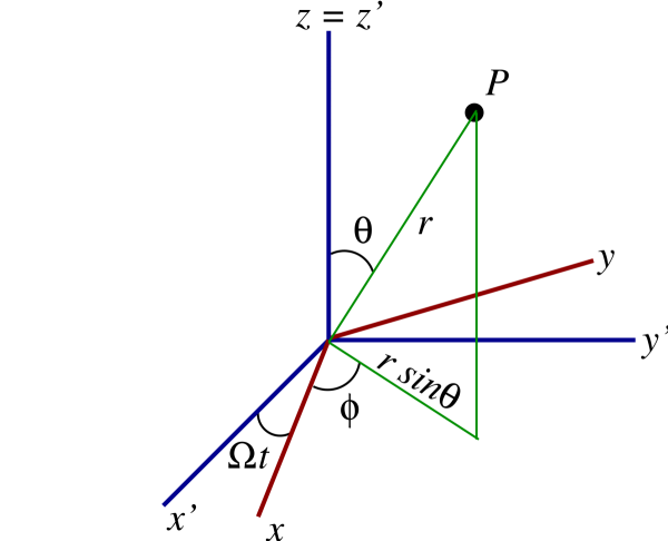
To work out the relationship between the coordinate systems we use, as a tool, the spherical coordinates $(r,\theta,\phi)$ and $(r',\theta',\phi')$ assigned to an arbitrary point $P$. Because the frames $S$ and $S'$ share the same origin, we have in fact that $r' = r$. And because they share also the same $z$ axis, we also have $\theta' = \theta$. The angles $\phi'$ and $\phi$ differ, however, and Fig.2.17 makes it clear that they are related by $\phi' = \phi + \Omega t$. We have
\[ x = r\sin\theta\cos\phi, \qquad y = r\sin\theta\sin\phi, \qquad z = r\cos\theta \]
and
\[ x' = r\sin\theta\cos\phi', \qquad y' = r\sin\theta\sin\phi', \qquad z' = r\cos\theta. \]
The relationship is obtained by substituting $\phi' = \phi + \Omega t$ into the previous expressions. It is a bit more efficient to first construct the complex combinations
\[ x + i y = r\sin\theta(\cos\phi + i \sin\phi) = r\sin\theta\, e^{i\phi} \]
and
\[ x' + i y' = r\sin\theta(\cos\phi' + i \sin\phi') = r\sin\theta\, e^{i\phi'}. \]
Then we have
\[ x' + i y' = r\sin\theta\, e^{i(\phi + \Omega t)} = e^{i\Omega t} r\sin\theta\, e^{i\phi}, \]
or
\begin{equation} x' + i y' = e^{i\Omega t} (x + i y). \tag{2.7.1} \end{equation}
When fully expanded, this is
\begin{equation} x' = x\cos\Omega t - y\sin\Omega t, \qquad y' = y\cos\Omega t + x\sin\Omega t, \qquad z' = z. \tag{2.7.2} \end{equation}
Exercise 2.19: Verify that Eq.(2.7.2) follows from Eq.(2.7.1). Then work out the inverse transformation, $(x',y',z') \to (x,y,z)$.
A particle moving in the rotating frame $S$ with a position vector $\boldsymbol{r}(t) = [x(t),y(t),z(t)]$ moves in the inertial frame $S'$ with a position vector $\boldsymbol{r'}(t) = [x'(t),y'(t),z'(t)]$; these are related by the transformation of Eq.(2.7.2). The components of the velocity vectors are then related by
\begin{align} \dot{x}' &= \dot{x} \cos\Omega t - \dot{y} \sin\Omega t - \Omega(x \sin\Omega t + y \cos\Omega t), \\ \dot{y}' &= \dot{y} \cos\Omega t + \dot{x} \sin\Omega t - \Omega(y \sin\Omega t - x \cos\Omega t), \\ \dot{z}' &= \dot{z}. \end{align}
After a fairly laborious calculation, we find that the squared velocity, as measured in the inertial frame, is
\begin{align} v^{\prime 2} &= \dot{x}^{\prime 2} + \dot{y}^{\prime 2} + \dot{y}^{\prime 2} \nonumber \\ &= \dot{x}^2 + \dot{y}^2 + \dot{z}^2 - 2\Omega(y \dot{x} - x\dot{y}) + \Omega^2 (x^2 + y^2). \tag{2.7.3} \end{align}
The particle's kinetic energy is then $T = \frac{1}{2} m v^{\prime 2}$. It contains a contribution from $\boldsymbol{\dot{r}}$, the particle's velocity vector as measured in the rotating frame, and contributions from the rotational motion of the frame (the terms that involve $\Omega$).
Exercise 2.20: Verify Eq.(2.7.3). You will save yourself some work if you use the trick of forming complex combinations.
The particle's potential energy can be expressed in terms of the inertial coordinates $(x',y',z')$, but after the transformation of Eq.(2.7.2) it becomes a function of the rotating coordinates $(x,y,z)$. Denoting this function $V(x,y,z)$, we find that the particle's Lagrangian is
\begin{equation} L = \frac{1}{2} m (\dot{x}^2 + \dot{y}^2 + \dot{z}^2) - m\Omega(y \dot{x} - x\dot{y}) + \frac{1}{2} m \Omega^2 (x^2 + y^2) - V(x,y,z). \tag{2.7.4} \end{equation}
The equations of motion for the particle are then obtained by substituting this into the EL equations for $x$, $y$, and $z$.
The computations that lead to the equations of motion will be left as an exercise for the reader. We find
\begin{align} m\ddot{x} &= -\frac{\partial V}{\partial x} + 2m\Omega \dot{y} + m\Omega^2 x, \tag{2.7.5} \\ m\ddot{y} &= -\frac{\partial V}{\partial y} - 2m\Omega \dot{x} + m\Omega^2 y, \tag{2.7.6} \\ m\ddot{z} &= -\frac{\partial V}{\partial z}. \tag{2.7.7} \end{align}
These equations can be expressed in vectorial form if we introduce the angular-velocity vector $\boldsymbol{\Omega}$, defined by
\begin{equation} \boldsymbol{\Omega} = \Omega \boldsymbol{\hat{z}} = [0,0,\Omega]. \tag{2.7.8} \end{equation}
The vectorial form is
\begin{equation} m \ddot{\boldsymbol{r}} = \boldsymbol{F}_{\rm applied} + \boldsymbol{F}_{\rm Coriolis} + \boldsymbol{F}_{\rm centrifugal}, \tag{2.7.9} \end{equation}
where
\begin{equation} \boldsymbol{F}_{\rm applied} = -\boldsymbol{\nabla} V \tag{2.7.10} \end{equation}
is the true applied force on the particle, given by the gradient of the potential energy, while
\begin{equation} \boldsymbol{F}_{\rm Coriolis} = 2 m \boldsymbol{\dot{r}} \times \boldsymbol{\Omega} = [2m\Omega \dot{y}, -2m\Omega \dot{x}, 0] \tag{2.7.11} \end{equation}
and
\begin{equation} \boldsymbol{F}_{\rm centrifugal} = m \boldsymbol{\Omega} \times (\boldsymbol{r} \times \boldsymbol{\Omega}) = [m\Omega^2 x, m\Omega^2 y, 0] \tag{2.7.12} \end{equation}
are fictitious forces that arise because the reference frame $S$ is not an inertial frame (refer back to the discussion of Sec.1.1). The Coriolis force is linear in the angular velocity $\Omega$, and it depends on the particle's velocity vector $\boldsymbol{\dot{r}}$; its effect on the particle depends on its state of motion. The centrifugal force is quadratic in $\Omega$, and it depends only on the position vector $\boldsymbol{r}$; this is always an outward force that points away from the centre of motion.
Exercise 2.21: Verify that Eqs.(2.7.5)--(2.7.7) follow from the Lagrangian of Eq.(2.7.4).
Exercise 2.22: Show that Eqs.(2.7.5)--(2.7.7) are equivalent to the vectorial equation (2.7.9), together with the definitions of Eqs.(2.7.10)--(2.7.12).
2.7.2 Case Study #1: Particle Attached to a Spring
As our first application of the rotating-frame formalism we examine a particle attached to a linear spring that is free to rotate around the $z$ axis. The particle is thus subjected to the potential $V = \frac{1}{2} k (x^2 + y^2)$, which we write in the alternative form
\begin{equation} V = \frac{1}{2} m \omega^2 (x^2 + y^2), \tag{2.7.13} \end{equation}
in which $\omega^2 \equiv k/m$ is a stand-in for the spring constant $k$. For simplicity we assume that the particle is confined to the $x$-$y$ plane and we set, accordingly, $z = \dot{z} = 0$ in all equations.
The equations of motion of Eqs.(2.7.5) and (2.7.6) become
\begin{equation} \ddot{x} = 2\Omega \dot{y} + (\Omega^2-\omega^2) x, \qquad \ddot{y} = -2\Omega \dot{x} + (\Omega^2-\omega^2) y. \tag{2.7.14} \end{equation}
Let us first analyze these equations in the limit of no rotation, $\Omega = 0$. In this case they reduce to $\ddot{x} = -\omega^2 x$ and $\ddot{y} = -\omega^2 y$, the equations of simple harmonic motion. The general solution to the equations of motion is then
\begin{equation} x_{\Omega = 0}(t) = a \cos(\omega t + \alpha), \qquad y_{\Omega = 0}(t) = b \cos(\omega t + \beta). \tag{2.7.15} \end{equation}
The four constants $a$, $b$, $\alpha$, and $\beta$ can be related to the four initial values $x(0)$, $\dot{x}(0)$, $y(0)$, and $\dot{y}(0)$. Equations (2.7.5) are parametric equations for the motion of the particle in the $x$-$y$ plane, and it is easy to show that the trajectory is elliptical.
To analyze the equations in the general case ($\Omega \neq 0$) we once more employ the clever trick of forming complex combinations. We introduce $\xi = x + iy$ and we combine the two equations (2.7.14) into a single equation for $\xi$:
\begin{align} \ddot{\xi} &= \ddot{x} + i \ddot{y} \\ &= 2\Omega (\dot{y} - i \dot{x}) + (\Omega^2-\omega^2)(x + iy) \\ &= -2i\Omega (\dot{x} + i \dot{y}) + (\Omega^2-\omega^2)(x + iy), \end{align}
or
\begin{equation} \ddot{\xi} + 2i\Omega \dot{\xi} - (\Omega^2-\omega^2) \xi = 0. \tag{2.7.16} \end{equation}
To find solutions to this equation we use a trial expression of the form $\xi = c e^{i\lambda t}$, where $c$ and $\lambda$ are complex constants. Substitution into Eq.(2.7.16) produces a quadratic equation for $\lambda$,
\[ \lambda^2 + 2\Omega \lambda + (\Omega^2 - \omega^2) = 0, \]
which factorizes as
\[ (\lambda + \Omega + \omega)(\lambda + \Omega - \omega) = 0. \]
The solutions, obviously, are $\lambda = -(\Omega \pm \omega)$, and the general solution for $\xi$ is
\[ \xi = c_1 e^{-i(\Omega + \omega)t} + c_2 e^{-i(\Omega - \omega)t}, \]
or
\[ \xi = e^{-i\Omega t} \bigl( c_1 e^{-i\omega t} + c_2 e^{i\omega t} \bigr), \]
where $c_1$ and $c_2$ are complex numbers.
To help us understand what we have just found, we observe that if we let $\Omega$ go to zero, our general solution for $\xi$ becomes $c_1 e^{-i\omega t} + c_2 e^{i\omega t}$. This is the solution in the limit of no rotation, and this must be equal to $x_{\Omega=0} + i y_{\Omega=0}$, which was given by Eq.(2.7.15) above. So we can write our general solution as
\begin{equation} \xi(t) = e^{-i\Omega t} \bigl[ x_{\Omega=0}(t) + i y_{\Omega=0}(t) \bigr]. \tag{2.7.17} \end{equation}
Written in full, this is
\begin{equation} x(t) = x_{\Omega=0}(t) \cos\Omega t + y_{\Omega=0}(t) \sin\Omega t, \qquad y(t) = y_{\Omega=0}(t) \cos\Omega t - x_{\Omega=0}(t) \sin\Omega t. \tag{2.7.18} \end{equation}
What is the meaning of these results? The answer is simple. Comparison with the transformations of Eqs.(2.7.1) and (2.7.2) shows that the motion of the particle on the turntable is a rotated version of the motion that would take place in an inertial frame; the rotation angle is here $-\Omega t$ instead of $+\Omega t$. This is easy to understand: The motion $x_{\Omega=0}(t)$, $y_{\Omega=0}(t)$ is what the particle would do in an inertial frame; because, however, we are measuring this motion in a rotating frame, we see a rotated version of the inertial motion. This conclusion is confirmed by substituting our solution of Eqs.(2.7.17), (2.7.18) into Eqs.(2.7.1), (2.7.2); the result is
\[ x'(t) = x_{\Omega=0}(t), \qquad y'(t) = y_{\Omega=0}(t), \]
as expected. The motion of the particle as measured in the rotating frame is shown in Fig.2.18 for three selected values of $\Omega$.
Exercise 2.23: Fill in the mathematical gaps that were left behind in the presentation of this subsection.
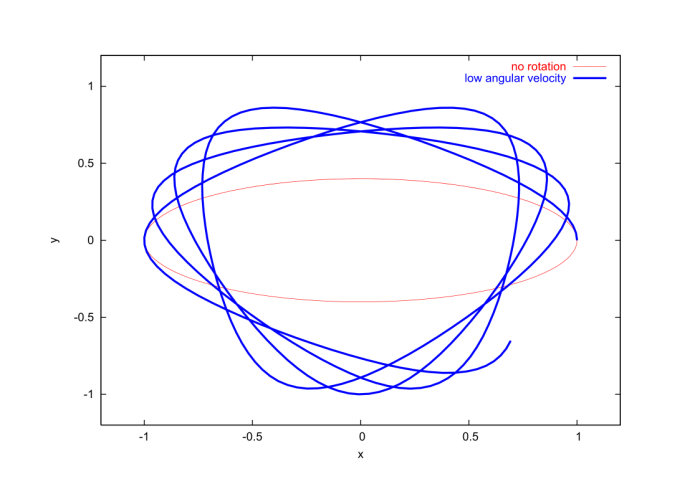
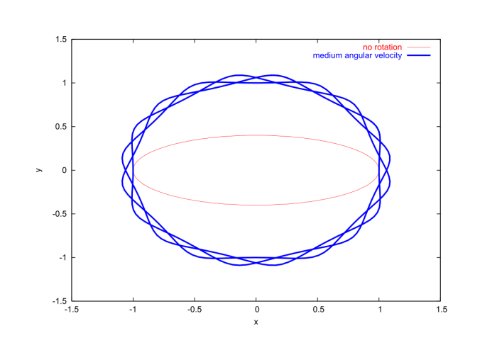
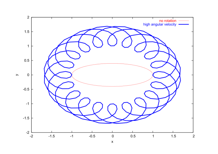
2.7.3 Motion on a Rotating Earth. Kinematics
We wish to describe the motion of a mechanical system from the point of view of an observer attached to a point $P$ on the surface of a rotating Earth. This will be done with the help of a Cartesian frame $(x,y,z)$ whose origin will be at $P$, and which will rotate along with the Earth. We will construct this Cartesian coordinate system in two stages. In the first stage we will momentarily assume that the Earth does not, in fact, rotate around its polar axis; in the second stage we will incorporate the rotation.
We first place a Cartesian frame $(x',y',z')$ at the centre of the nonrotating Earth. Neglecting the Earth's motion around the Sun, we consider this to be an inertial frame. Our end goal in this subsection is to relate $(x,y,z)$, the local frame at $P$, to the inertial frame $(x',y',z')$. Our first step toward this goal is to introduce the spherical coordinates $(r',\theta',\phi')$, which are related to the original Cartesian coordinates by
\[ x' = r'\sin\theta'\cos\phi', \qquad y' = r'\sin\theta'\sin\phi', \qquad z' = r'\cos\theta'. \]
As shown in Fig.2.19, our point $P$ on the Earth's surface is at a distance $r' = R$ from the centre, and its position on the sphere is determined by the colatitude $\theta'$ and the longitude $\phi'$. (The latitude $\lambda'$ is related to the colatitude by $\lambda' = \frac{\pi}{2} - \theta'$; thus the colatitude of the equator is $90^\circ$ while its latitude is $0^\circ$.) Because the Earth is not yet rotating the longitude of $P$ is a fixed angle; when we later incorporate the rotation into the picture we will put $\phi' = \Omega t$, with $\Omega$ denoting the Earth's angular velocity.
The spherical coordinates come with a set of basis vectors $(\boldsymbol{\hat{r}}', \boldsymbol{\hat{\theta}}', \boldsymbol{\hat{\phi}}')$. Following the discussion of Sec.1.2, we derive that these vectors are related to the Cartesian basis $(\boldsymbol{\hat{x}}', \boldsymbol{\hat{y}}', \boldsymbol{\hat{z}}')$ by
\begin{align} \boldsymbol{\hat{r}'} &= \frac{\partial \boldsymbol{r'}}{\partial r'} = \sin\theta'\cos\phi'\, \boldsymbol{\hat{x}'} + \sin\theta'\sin\phi' \boldsymbol{\hat{y}'}+ \cos\theta'\, \boldsymbol{\hat{z}}', \tag{2.7.19} \\ \boldsymbol{\hat{\theta}}' &= \frac{1}{r'}\frac{\partial \boldsymbol{\hat{r'}}}{\partial \theta'} = \cos\theta'\cos\phi'\, \boldsymbol{\hat{x}}' + \cos\theta'\sin\phi' \boldsymbol{\hat{y}}' - \sin\theta'\, \boldsymbol{\hat{z}}', \tag{2.7.20} \\ \boldsymbol{\hat{\phi}}' &= \frac{1}{r'\sin\theta'} \frac{\partial \boldsymbol{r'}}{\partial \phi'} = -\sin\phi'\, \boldsymbol{\hat{x}}' + \cos\phi' \boldsymbol{\hat{y}}'. \tag{2.7.21} \end{align}
Here $\boldsymbol{r'}$ is the position vector expressed in terms of the spherical coordinates,
\begin{equation} \boldsymbol{r'} = r'\sin\theta'\cos\phi'\, \boldsymbol{\hat{x}}' + r'\sin\theta'\sin\phi'\, \boldsymbol{\hat{y}}' + r'\cos\theta'\, \boldsymbol{\hat{z}}'. \tag{2.7.22} \end{equation}
The position vector of the point $P$ on the surface is
\begin{equation} \boldsymbol{R} = R\sin\theta'\cos\phi'\, \boldsymbol{\hat{x}}' + R\sin\theta'\sin\phi'\, \boldsymbol{\hat{y}}' + R\cos\theta'\, \boldsymbol{\hat{z}}'. \tag{2.7.23} \end{equation}

The spherical coordinates are useful to specify the position of the laboratory on the Earth's surface, but they are not so useful to describe the motion of mechanical bodies that would take place in this laboratory. For this purpose we introduce another Cartesian frame $(x,y,z)$ whose origin will be at $P$. The orientation of this frame will be set by the directions of the basis vectors $(\boldsymbol{\hat{r}}', \boldsymbol{\hat{\theta}}', \boldsymbol{\hat{\phi}}')$. Thus, the $z$ axis will point away from the surface, and will be aligned in the direction of $\boldsymbol{\hat{r}}'$; the $x$ axis will point in the southern direction, and will be aligned in the direction of $\boldsymbol{\hat{\theta}}'$; and the $y$ axis will point in the eastern direction, and will be aligned in the direction of $\boldsymbol{\hat{\phi}}'$. We therefore set
\begin{equation} \boldsymbol{\hat{x}} = \boldsymbol{\hat{\theta}}', \qquad \boldsymbol{\hat{y}} = \boldsymbol{\hat{\phi}}', \qquad \boldsymbol{\hat{z}} = \boldsymbol{\hat{r}}'. \tag{2.7.24} \end{equation}
The situation is illustrated in Fig.2.20.
We denote by $\boldsymbol{r}$ the position vector of a particle located at a point $Q$ near the surface of the Earth, relative to the surface point $P$ to which our frame $(x,y,z)$ is attached. As usual we will resolve this vector in the basis $(\boldsymbol{\hat{x}},\boldsymbol{\hat{y}},\boldsymbol{\hat{z}})$ and identify the components with the particle's coordinates. We have
\[ \boldsymbol{r} = x\, \boldsymbol{\hat{x}} + y\, \boldsymbol{\hat{y}} + z\, \boldsymbol{\hat{z}}, \]
and if we involve Eq.(2.7.24) we obtain
\[ \boldsymbol{r} = x\, \boldsymbol{\hat{\theta}}' + y\, \boldsymbol{\hat{\phi}}' + z\, \boldsymbol{\hat{r}}'. \]
If we now substitute Eqs.(2.7.19)--(2.7.21) and rearrange what we get, we find
\begin{align} \boldsymbol{r} &= (x\cos\theta'\cos\phi' - y\sin\phi' + z\sin\theta'\cos\phi') \boldsymbol{\hat{x}}' + (x\cos\theta'\sin\phi' + y\cos\phi' + z\sin\theta'\sin\phi') \boldsymbol{\hat{y}}' + (-x\sin\theta' + z\cos\theta') \boldsymbol{\hat{z}}'. \end{align}
The position vector of the particle relative to the centre of the Earth is $\boldsymbol{R} + \boldsymbol{r}$. According to Eq.(2.7.23) and our previous result, this is
\begin{align} \boldsymbol{R} + \boldsymbol{r} &= \bigl[ x\cos\theta'\cos\phi' - y\sin\phi' + (R+z)\sin\theta'\cos\phi' \bigr] \boldsymbol{\hat{x}}' + \bigl[ x\cos\theta'\sin\phi' + y\cos\phi' + (R+z)\sin\theta'\sin\phi' \bigr] \boldsymbol{\hat{y}}' + \bigl[ -x\sin\theta' + (R+z)\cos\theta'\bigr] \boldsymbol{\hat{z}}'. \end{align}
The components of this vector in the original Cartesian basis $(\boldsymbol{\hat{x}}',\boldsymbol{\hat{y}}',\boldsymbol{\hat{z}}')$ are the original Cartesian coordinates $(x',y',z')$ of the particle at $Q$. We have obtained, therefore, the transformation
\begin{align} x' &= \cos\theta'\cos\phi' - y\sin\phi' + (R+z)\sin\theta'\cos\phi', \tag{2.7.25} \\ y' &= x\cos\theta'\sin\phi' + y\cos\phi' + (R+z)\sin\theta'\sin\phi', \tag{2.7.26} \\ z' &= - x\sin\theta' + (R+z)\cos\theta', \tag{2.7.27} \end{align}
between the two systems of Cartesian coordinates.
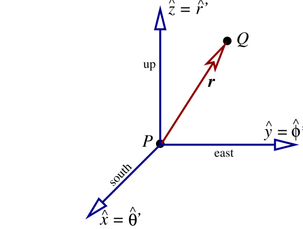
Our considerations so far have relied on the fiction of a nonrotating Earth. To finally incorporate its rotation into the picture we set $\phi' = \Omega t$ into Eqs.(2.7.25)--(2.7.27), with $\Omega$ denoting the Earth's angular velocity. We also, at the same time, fix the colatitude of our laboratory to $\theta' = \alpha$. The transformation between the local rotating frame $(x,y,z)$ and the original inertial frame $(x',y',z')$ is finally given by
\begin{align} x' &= x\cos\alpha\cos\Omega t - y\sin\Omega t + (R+z)\sin\alpha\cos\Omega t, \tag{2.7.28} \\ y' &= x\cos\alpha\sin\Omega t + y\cos\Omega t + (R+z)\sin\alpha\sin\Omega t, \tag{2.7.29} \\ z' &= - x\sin\alpha + (R+z)\cos\alpha. \tag{2.7.30} \end{align}
We recall that $R$ is the Earth's radius, that the $x$ direction points due south, that the $y$ direction points due east, and that the $z$ direction points up, away from the surface.
Exercise 2.24: Fill in the mathematical gaps that were left behind in the presentation of this subsection.
2.7.4 Motion on a Rotating Earth. Dynamics
Having established the transformation of Eqs.(2.7.28)--(2.7.30) we may now turn to the task of describing the dynamics of a particle as viewed in the local rotating frame. The particle's coordinates $(x,y,z)$ are changing with time and we let $(\dot{x},\dot{y},\dot{z})$ denote the components of the velocity vector in the local rotating frame. In the inertial frame, according to Eqs.(2.7.28)--(2.7.30), the components of the velocity vector are
\begin{align} \dot{x}' &= \dot{x} \cos\alpha\cos\Omega t - \dot{y} \sin\Omega t + \dot{z}\sin\alpha\cos\Omega t - \Omega\bigl[ x\cos\alpha\sin\Omega t + y\cos\Omega t + (R+z)\sin\alpha\sin\Omega t \bigr], \\ \dot{y}' &= \dot{x} \cos\alpha\sin\Omega t + \dot{y}\cos\Omega t + \dot{z}\sin\alpha\sin\Omega t + \Omega\bigl[ x\cos\alpha\cos\Omega t - y\sin\Omega t + (R+z)\sin\alpha\cos\Omega t\bigr], \\ \dot{z}' &= -\dot{x}\sin\alpha + \dot{z}\cos\alpha. \end{align}
A fairly laborious calculation then returns the squared velocity; we find
\begin{align} v^{\prime 2} &= \dot{x}^2 + \dot{y}^2 + \dot{z}^2 + 2\Omega \Bigl\{ \bigl[ (R+z) \dot{y} - y \dot{z} \bigr] \sin\alpha + \bigl[ x \dot{y} - y \dot{x} \bigr] \cos\alpha \Bigr\} \nonumber + \Omega^2 \Bigl\{ \bigl[ x\cos\alpha + (R+z) \sin\alpha \bigr]^2 + y^2 \Bigr\}. \tag{2.7.31} \end{align}
The particle's kinetic energy is $T = \frac{1}{2} m v^{\prime 2}$. Again (as in Sec.2.7.1) we see that the kinetic energy has a contribution from the particle's motion within the local rotating frame, and contributions from the motion of the frame; these depend on $\Omega$ and the laboratory's colatitude $\alpha$.
Exercise 2.25: Verify Eq.(2.7.31).
The particle's potential energy comes from two different sources, which we choose to distinguish in this subsection. The first is the Earth's gravity, and this contribution to the potential energy is $V_{\rm gravity} = m g z$, as usual. The second contribution comes from all the other forces acting on the particle; we write this as $V_{\rm other} = U$. The total potential energy is then
\begin{equation} V = mgz + U(x,y,z). \tag{2.7.32} \end{equation}
The particle's Lagrangian is, finally,
\begin{align} L &= \frac{1}{2} m (\dot{x}^2 + \dot{y}^2 + \dot{z}^2) + m\Omega \Bigl\{ \bigl[ (R+z) \dot{y} - y \dot{z} \bigr] \sin\alpha + \bigl[ x \dot{y} - y \dot{x} \bigr] \cos\alpha \Bigr\} \nonumber + \frac{1}{2} m \Omega^2 \Bigl\{ \bigl[ x\cos\alpha + (R+z) \sin\alpha \bigr]^2 + y^2 \Bigr\} - mgz - U(x,y,z). \tag{2.7.33} \end{align}
The equations of motion in the local rotating frame are obtained by substituting this into the EL equations.
Omitting the detail of the calculations, the equations of motion are
\begin{align} m \ddot{x} &= -\frac{\partial U}{\partial x} + 2m\Omega \dot{y} \cos\alpha + m\Omega^2 \bigl[ x\cos\alpha + (R+z)\sin\alpha \bigr] \cos\alpha, \tag{2.7.34} \\ m \ddot{y} &= -\frac{\partial U}{\partial y} - 2m\Omega (\dot{x} \cos\alpha + \dot{z}\sin\alpha) + m\Omega^2 y, \tag{2.7.35} \\ m \ddot{z} &= -mg -\frac{\partial U}{\partial z} + 2m\Omega \dot{y} \sin\alpha + m\Omega^2 \bigl[ x\cos\alpha + (R+z)\sin\alpha \bigr] \sin\alpha. \tag{2.7.36} \end{align}
These equations can be expressed in vectorial form if we introduce the angular-momentum vector $\boldsymbol{\Omega}$. This is given by $\boldsymbol{\Omega} = \Omega \boldsymbol{\hat{z}}'$, and in the local rotating frame we have the components $\Omega_x = \boldsymbol{\Omega} \cdot \boldsymbol{\hat{x}} = \Omega \boldsymbol{\hat{z}}' \cdot \boldsymbol{\hat{\theta}}' = -\Omega\sin\alpha$, $\Omega_y = \boldsymbol{\Omega} \cdot \boldsymbol{\hat{y}} = \Omega \boldsymbol{\hat{z}}' \cdot \boldsymbol{\hat{\phi}}' = 0$, and $\Omega_z = \boldsymbol{\Omega} \cdot \boldsymbol{\hat{z}} = \Omega \boldsymbol{\hat{z}}' \cdot \boldsymbol{\hat{r}}' = \Omega\cos\alpha$. The vector is therefore given by
\begin{equation} \boldsymbol{\Omega} = -\Omega\sin\alpha\, \boldsymbol{\hat{x}} + \Omega\cos\alpha\, \boldsymbol{\hat{z}} = [-\Omega\sin\alpha, 0, \Omega\cos\alpha] \tag{2.7.37} \end{equation}
in the local rotating frame. We also re-express the vector $\boldsymbol{R}$ of Eq.(2.7.23) as
\begin{equation} \boldsymbol{R} = R\boldsymbol{\hat{z}} = [0,0,R]; \tag{2.7.38} \end{equation}
this gives the position of the laboratory relative to the Earth's centre.
The vectorial equation is
\begin{equation} m \ddot{\boldsymbol{r}} = m \boldsymbol{g} + \boldsymbol{F}_{\rm applied} + \boldsymbol{F}_{\rm Coriolis} + \boldsymbol{F}_{\rm centrifugal}, \tag{2.7.39} \end{equation}
where $\boldsymbol{g} = -g\boldsymbol{\hat{z}} = [0,0,-g]$ is the acceleration of gravity, $\boldsymbol{F}_{\rm applied} = -\boldsymbol{\nabla} U$ is the net force coming from all other interactions,
\begin{equation} \boldsymbol{F}_{\rm Coriolis} = 2 m \boldsymbol{\dot{r}} \times \boldsymbol{\Omega} \tag{2.7.40} \end{equation}
is the Coriolis force, and
\begin{equation} \boldsymbol{F}_{\rm centrifugal} = m\boldsymbol{\Omega} \times \bigl[ (\boldsymbol{R} + \boldsymbol{r}) \times \boldsymbol{\Omega} \bigr] \tag{2.7.41} \end{equation}
is the centrifugal force. In Eq.(2.7.39), $m\boldsymbol{g}$ and $\boldsymbol{F}_{\rm applied}$ are genuine forces acting on the particle, while $\boldsymbol{F}_{\rm Coriolis}$ and $\boldsymbol{F}_{\rm centrifugal}$ are fictitious forces that arise from the rotational motion of the frame.
Exercise 2.26: Verify that Eqs.(2.7.34)--(2.7.36) follow from the Lagrangian of Eq.(2.7.33).
Exercise 2.27: Show that Eqs.(2.7.34)--(2.7.36) are equivalent to the vectorial equation (2.7.39), together with the definitions of Eqs.(2.7.37), (2.7.38), (2.7.40), and (2.7.41).
2.7.5 Case Study #2: Particle Released from Rest
To gain some insight into the effects of Earth's rotation we shall determine what happens to a particle that is released from rest at a great height $h$ in the Earth's gravitational field. Because the Earth's rotation is quite slow, it will be sufficient to work consistently to first order in the angular velocity $\Omega$. We will therefore neglect all terms of order $\Omega^2$ in the equations of motion; this means that we will keep the Coriolis term, but discard the centrifugal term.
At this level of accuracy the equations of motion (2.7.34)--(2.7.36) reduce to
\begin{equation} \ddot{x} = 2\Omega \dot{y} \cos\alpha, \qquad \ddot{y} = -2\Omega (\dot{x} \cos\alpha + \dot{z} \sin\alpha), \qquad \ddot{z} = -g + 2\Omega \dot{y} \sin\alpha. \tag{2.7.42} \end{equation}
We impose the initial conditions $x(0) = y(0) = 0$, $z(0) = h$, as well as $\dot{x}(0) = \dot{y}(0) = \dot{z}(0) = 0$.
We shall solve Eqs.(2.7.42) by the method of successive approximations. We first express the particle's coordinates $x(t)$, $y(t)$, and $z(t)$ as formal expansions in powers of $\Omega$. Thus,
\[ x(t) = x_0(t) + \Omega x_1(t) + \cdots, \quad y(t) = y_0(t) + \Omega y_1(t) + \cdots, \quad z(t) = z_0(t) + \Omega z_1(t) + \cdots. \]
In terms of these new quantities the initial conditions become $x_0(0) = y_0(0) = 0$, $z_0(0) = h$, $x_1(0) = y_1(0) = z_1(0) = 0$, as well as $\dot{x}_0(0) = \dot{y}_0(0) = \dot{z}_0(0) = \dot{x}_1(0) = \dot{y}_1(0) = \dot{z}_1(0) = 0 $. Substituting the expansions into Eq.(2.7.42) yields
\begin{align} \ddot{x}_0 + \Omega \ddot{x}_1 + \cdots &= 2\Omega (\dot{y}_0 + \cdots)\cos\alpha, \\ \ddot{y}_0 + \Omega \ddot{y}_1 + \cdots &= -2\Omega (\dot{x}_0 \cos\alpha + \dot{z}_0 \sin\alpha + \cdots), \\ \ddot{z}_0 + \Omega \ddot{z}_1 + \cdots &= -g + 2\Omega (\dot{y}_0 + \cdots)\sin\alpha. \end{align}
Equating powers of $\Omega$ produces the set of equations
\[ \ddot{x}_0 = 0, \qquad \ddot{y}_0 = 0, \qquad \ddot{z}_0 = -g, \] \[ \ddot{x}_1 = 2\dot{y}_0 \cos\alpha, \qquad \ddot{y}_1 = -2\dot{x}_0 \cos\alpha - 2\dot{z}_0 \sin\alpha, \qquad \ddot{z}_1 = 2\dot{y}_0\sin\alpha. \]
The zeroth-order equations are easy to solve. In view of the initial conditions, the solutions are
\[ x_0(t) = 0, \qquad y_0(t) = 0, \qquad z_0(t) = h - \frac{1}{2} g t^2. \]
With $\dot{x}_0 = \dot{y}_0 = 0$ and $\dot{z}_0 = -gt$ the first-order equations become
\[ \ddot{x}_1 = 0, \qquad \ddot{y}_1 = 2 gt \sin\alpha, \qquad \ddot{z}_1 = 0. \]
These equations also are easy to solve. Taking once more the initial conditions into account, we find that the solutions are
\[ x_1(t) = 0, \qquad y_1(t) = \frac{1}{3} g t^3 \sin\alpha, \qquad z_1(t) = 0. \]
The complete solution to the equations of motion is therefore
\begin{align} x(t) &= 0 + O(\Omega^2), \tag{2.7.43} \\ y(t) &= \frac{1}{3} (g \Omega \sin\alpha) t^3 + O(\Omega^2), \tag{2.7.44} \\ z(t) &= h - \frac{1}{2} g t^2 + O(\Omega^2). \tag{2.7.45} \end{align}
Observe that the factor $g\Omega\sin\alpha$ is positive for any colatitude $\alpha$, except at the North and South poles where it is zero. The fact that $y$ increases during the motion means that the particle, which would just fall straight down in the absence of rotation, is in fact drifting away in the eastward direction.
The time required for the particle to hit the ground is $t = (2h/g)^{1/2}$, and by this time to total eastward displacement is
\begin{equation} y_{\rm total} = \frac{1}{3} (g \Omega \sin\alpha) \biggl( \frac{2h}{g} \biggr)^{3/2}. \tag{2.7.46} \end{equation}
If the object is released from a height of 100 m at Guelph's colatitude (approximately $47^\circ$), this amounts to approximately 1.6 cm. The Coriolis force produces a rather small effect.
Exercise 2.28: Compute this number.
2.7.6 Case Study #3: Foucalt's Pendulum
A dramatic demonstration of Earth's rotation came from Foucault's celebrated pendulum, which was first displayed in front of an audience at the Observatoire de Paris in 1851. The idea is that while the Earth rotates the pendulum keeps oscillating in a fixed plane as viewed from an inertial frame; as seen from the Earth's rotating frame, however, it is the pendulum that appears to be rotating. More precisely stated, as viewed in the local rotating frame the pendulum is swinging in a plane which rotates at a steady rate $\Omega_{\rm plane}$; this is directly related to $\Omega$, the rate at which the Earth itself is rotating.
In this last application we will examine the motion of a pendulum in the local rotating frame. We aim to calculate $\Omega_{\rm plane}$, in an approximation in which we neglect the centrifugal effects (which are proportional to $\Omega^2$) but retain the Coriolis effects (which are proportional to $\Omega$), and in an approximation in which the amplitude of the pendulum's oscillations is assumed to be small.
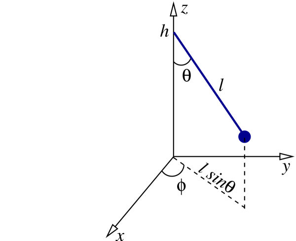
In the spirit of Lagrangian mechanics we will use the generalized coordinates $\theta$ and $\phi$ to describe the motion of the pendulum, as illustrated in Fig.2.21. (Notice that $\theta$, as defined here, is not the standard spherical coordinate.) The relation between these generalized coordinates and the original Cartesian system $(x,y,z)$ is given by
\begin{equation} x = \ell\sin\theta\cos\phi, \qquad y = \ell\sin\theta\sin\phi, \qquad z = h - \ell\cos\theta. \tag{2.7.47} \end{equation}
The pendulum has a constant length $\ell$, and its pivot point is attached at a height $h$ above the Earth's surface. As usual we introduce the quantity
\begin{equation} \omega^2 = g/\ell, \tag{2.7.48} \end{equation}
and we will use it instead of $g$.
The two degrees of freedom of the pendulum are represented by the angles $\theta$ and $\phi$. The first angle, $\theta$, is the usual swing angle of the pendulum. In the absence of rotation, the pendulum would swing in a fixed plane, and $\phi$ would stay constant; in this situation there would be a single degree of freedom. But as we shall see, the Earth's rotation will force $\phi$ to change steadily with time, and the plane of the pendulum will rotate in the $x$-$y$ plane; in this situation there are two degrees of freedom, and $\phi$ is the rotation angle of the swing plane.
According to Eq.(2.7.47) the pendulum's velocity vector has the components
\begin{align} \dot{x} &= \ell\cos\theta\cos\phi\, \dot{\theta} - \ell\sin\theta\sin\phi\, \dot{\phi}, \\ \dot{y} &= \ell\cos\theta\sin\phi\, \dot{\theta} + \ell\sin\theta\cos\phi\, \dot{\phi}, \\ \dot{z} &= \ell\sin\theta\, \dot{\theta}. \end{align}
It follows that the squared velocity is
\[ v^2 = \ell^2 \dot{\theta}^2 + \ell^2\sin^2\theta\, \dot{\phi}^2. \]
We make this substitution, along with $z = h-\ell\cos\theta$, into the Lagrangian of Eq.(2.7.33), and we allow ourselves (once more) to neglect the centrifugal terms that are proportional to $\Omega^2$. This yields
\begin{align} L &= \frac{1}{2} m \ell^2 (\dot{\theta}^2 + \sin^2\theta\, \dot{\phi}^2) + m\Omega \Bigl\{ \bigl[ (R+h-\ell\cos\theta) \dot{y} - y \dot{z} \bigr] \sin\alpha + \bigl[ x \dot{y} - y \dot{x} \bigr] \cos\alpha \Bigr\} - mg(h-\ell\cos\theta). \end{align}
In this Lagrangian we recognize a term $m\Omega(R+h)\dot{y}\sin\alpha$ and another term $-mgh$ that can both be discarded. We can omit the first term because it is the time derivative of the function $m\Omega(R+h)y\sin\alpha$, and as we have learned in Sec.2.5.3, such a term will not contribute to the equations of motion. And we can omit the second term for the simple reason that it is a constant; it will also contribute nothing to the equations of motion.
The Lagrangian simplifies to
\begin{align} L &= \frac{1}{2} m \ell^2 (\dot{\theta}^2 + \sin^2\theta\, \dot{\phi}^2) + m\Omega \Bigl\{ -\bigl[ \ell\cos\theta\, \dot{y} + y \dot{z} \bigr] \sin\alpha + \bigl[ x \dot{y} - y \dot{x} \bigr] \cos\alpha \Bigr\} + mg \ell \cos\theta. \end{align}
This becomes
\begin{align} L &= m\ell^2 \biggl\{ \frac{1}{2} \bigl( \dot{\theta}^2 + \sin^2\theta\, \dot{\phi}^2 \bigr) - \Omega\sin\alpha \bigl( \sin\phi\, \dot{\theta} + \sin\theta\cos\theta\cos\phi\, \dot{\phi} \bigr) \nonumber + \Omega\cos\alpha \sin^2\theta\, \dot{\phi} + \omega^2 \cos\theta \biggr\}, \tag{2.7.49} \end{align}
after involving the transformation between the Cartesian coordinates $(x,y,z)$ and our generalized coordinates $(\theta,\phi)$. This is the pendulum's Lagrangian, up to terms of order $\Omega^2$ that have been neglected.
Exercise 2.29: Verify Eq.(2.7.49).
We may simplify the Lagrangian further if we assume that the amplitude of the pendulum's oscillations is sufficiently small that we can use the approximations
\[ \sin\theta \simeq \theta, \qquad \cos\theta \simeq 1 - \frac{1}{2} \theta^2. \]
Neglecting all terms of order $\theta^3$ and higher, we obtain
\begin{align} L &=&m\ell^2 \biggl\{ \frac{1}{2} \bigl( \dot{\theta}^2 + \theta^2\, \dot{\phi}^2 \bigr) - \Omega\sin\alpha \bigl( \sin\phi\, \dot{\theta} + \theta\cos\phi\, \dot{\phi} \bigr) + \Omega\cos\alpha\, \theta^2 \dot{\phi} + \omega^2 \biggl(1 - \frac{1}{2} \theta^2 \biggr) \biggr\}. \end{align}
In this simplified Lagrangian we recognize a term proportional to
\[ \sin\phi\, \dot{\theta} + \theta\cos\phi\, \dot{\phi} = \frac{d}{dt} \Bigl( \theta\sin\phi \Bigr); \]
we can discard this term from the Lagrangian because this is a total time derivative. We may also remove the constant term $\omega^2$. After these simplifications, our final Lagrangian will be
\begin{equation} L = m\ell^2 \biggl\{ \frac{1}{2} \bigl( \dot{\theta}^2 + \theta^2\, \dot{\phi}^2 \bigr) + \Omega\cos\alpha\, \theta^2 \dot{\phi} - \frac{1}{2} \omega^2 \theta^2 \biggr\}. \tag{2.7.50} \end{equation}
This is the simplified Lagrangian for Foucault's pendulum, and it is valid in the limit of small swing angles.
The equations of motion are obtained by substituting the Lagrangian of Eq.(2.7.50) into the EL equations. Omitting all details, we find that the equation for $\theta$ is
\begin{equation} \ddot{\theta} + \omega^2 \theta - \dot{\phi}(\dot{\phi} + 2\Omega\cos\alpha) \theta = 0. \tag{2.7.51} \end{equation}
And the fact that the Lagrangian does not depend explicitly on $\phi$ implies that the (rescaled) generalized momentum
\begin{equation} p_\phi = \theta^2(\dot{\phi} + \Omega\cos\alpha) \tag{2.7.52} \end{equation}
is a constant of the motion.
Exercise 2.30: Verify that the EL equations produce Eqs.(2.7.51) and the statement that $p_\phi$, as defined by Eq.(2.7.52), is constant.
Solving Eq.(2.7.52) for $\dot{\phi}$ gives $\dot{\phi} = -\Omega\cos\alpha + p_\phi/\theta^2$. We see that unless $p_\phi = 0$, $\dot{\phi}$ would blow up as $\theta \to 0$, that is, whenever the pendulum crosses the $z$ axis. To eliminate this unphysical behaviour we set $p_\phi = 0$, so that
\begin{equation} \dot{\phi} = -\Omega\cos\alpha. \tag{2.7.53} \end{equation}
This is our key result. In the absence of rotation we would find that $\dot{\phi} = 0$, and we would conclude that the pendulum swings in a fixed plane, as we had foreseen at the beginning of this subsection. With the Earth's rotation, however, we find instead that $\dot{\phi} = -\Omega\cos\alpha$, and this means that the swing plane is rotating with a constant angular velocity given by
\begin{equation} \Omega_{\rm plane} = -\Omega\cos\alpha. \tag{2.7.54} \end{equation}
This is the Foucault effect.
When the pendulum is located in the northern hemisphere, we have that $\cos\alpha > 0$ and we find that $\Omega_{\rm plane} < 0$, so that the swing plane rotates clockwise. When, on the other hand, we go to the southern hemisphere, we have that $\cos\alpha < 0$ and $\Omega_{\rm plane} > 0$, so that the swing plane rotates counterclockwise. The Foucault effect is maximum at the poles, and it vanishes at the equator.
Exercise 2.31: Calculate $\Delta\phi$, the angular displacement of the swing plane after 1 hour, when the Foucault pendulum is located in Guelph (colatitude $47^\circ$).
Exercise 2.32: This is the laboratory component of the course. There is a Foucault pendulum in the foyer of the MacNaughton building, and you are asked to determine its value for $\Delta\phi$. Measure the angular position of the swing plane when you first arrive in the Department of Physics, and record the time. Repeat the measurement when you are about to leave. Divide the difference in angular positions by the time interval measured in hours, and obtain your experimental value for $\Delta\phi$. How close is it to the theoretical value obtained in the previous exercise?
To finish off our discussion of the Foucault pendulum we return to Eq.(2.7.51), in which we substitute Eq.(2.7.53). The result is
\[ \ddot{\theta} + \omega^2 \theta - (-\Omega\cos\alpha)(+\Omega\cos\alpha) \theta = 0, \]
or
\[ \ddot{\theta} + (\omega^2 + \Omega^2\cos^2\alpha)\theta = 0. \]
This is the equation for simple harmonic motion, and it appears to indicate that the natural frequency of the pendulum is shifted from $\omega$ to $\sqrt{\omega^2 + \Omega^2\cos^2\alpha}$ by the Earth's rotation. This conclusion, however, is premature. In the course of our calculations we have consistently neglected all terms of order $\Omega^2$, starting with the Lagrangian of Eq.(2.7.49). We must continue to do so, and the previous equation must be approximated by
\begin{equation} \ddot{\theta} + \omega^2 \theta = 0. \tag{2.7.55} \end{equation}
This is still the equation for simple harmonic motion, with the original natural frequency $\omega = \sqrt{g/\ell}$. The general solution to this equation is $\theta(t) = \theta_0 \cos(\omega t + \delta)$, where $\theta_0$ and $\delta$ are constants.
To sum up, we have found that to first order in $\Omega$, the pendulum swings as a simple harmonic oscillator, but that it does so in a plane that rotates around the vertical direction with an angular velocity $\Omega_{\rm plane} = -\Omega\cos\alpha$.
2.8 Problems
- a) Find the curve $y(x)$ that passes through the endpoints $(0,0)$ and $(1,1)$ and minimizes the functional
\[I[y] = \int_0^1 \biggl[ \Bigl( \frac{dy}{dx} \Bigr)^2 - y^2 \biggr]\, dx. \]
b) What is the minimum value of the functional?
c) Evaluate $I[y]$ for a straight line that passes through the same two endpoints. Is this smaller or larger than your answer in part b)?
-
You are mounting an expedition to reach the other side of a volcano, and you wish to determine the path that will minimize the distance traveled. To perform this calculation you decide to use cylindrical coordinates $(\rho,\phi,z)$ and you model the volcano as the conical surface $z = 1 - \rho$. [The cylindrical coordinates are defined by $x=\rho\cos\phi$, $y=\rho\sin\phi$, and $z = z$.] You describe the path by the function $\rho(\phi)$ and let the angle $\phi$ range through the interval $-\frac{\pi}{2} \leq \phi \leq \frac{\pi}{2}$. The starting point of the expedition is $(\rho=1,\phi=-\frac{\pi}{2},z=0)$ and the end point is $(\rho=1,\phi=+\frac{\pi}{2},z=0)$. You wish to find the path $\rho(\phi)$ that minimizes the total distance traveled from this side of the volcano to the other side.
a) Prove that the functional that must be minimized is
\[s[\rho] = \int_{-\frac{\pi}{2}}^{\frac{\pi}{2}} \sqrt{2\rho^{\prime 2}+ \rho^2}\, d\phi,\]
where $\rho' = d\rho/d\phi$.
b) Find the differential equation that the minimal path must satisfy.
c) Show that
\[\rho(\phi) = \frac{\cos\Bigl( \frac{\pi}{2\sqrt{2}} \Bigr)}{\cos\Bigl(<\frac{\phi}{\sqrt{2}} \Bigr)}\]
is a solution to this differential equation, and that it satisfies the boundary conditions; conclude that this must be the minimal path. Produce a plot of $z = 1-\rho$ as a function of $\phi$.
d) Calculate the minimum distance $s_{\rm min}$. Compare this with the distance that would be traveled if the path were instead chosen to be $\rho(\phi) = 1$.
-
A bead of mass $m$ slides on a frictionless wire that is shaped in the form of a cycloid. This is described by the parametric equations
\[x = a(\theta - \sin\theta), \qquad y = a(1 + \cos\theta),\]
where $a$ is a constant and the parameter $\theta$ ranges through the interval $0 \leq \theta \leq 2\pi$. The bead is subjected to gravity, and it oscillates back and forth on the wire.
a) Using $\theta$ as a generalized coordinate, calculate the bead's Lagrangian.
b) Show that the equation of motion for the bead is
\[2(1-\cos\theta) \ddot{\theta} + \sin\theta\, \dot{\theta}^2 -\frac{g}{a} \sin\theta = 0.\]
c) Show that the transformation $u = \cos(\frac{1}{2} \theta)$ brings this equation to the much simpler form
\[\ddot{u} + \omega^2 u = 0,\]
and find an expression for $\omega$.
d) What is the period of the bead's oscillations?
-
A particle of mass $m$ moves on a paraboloid of revolution described by the equation
\[z = \frac{1}{a} \bigl( x^2 + y^2 \bigr),\]
where $a$ is a constant (see the figure). The particle is subjected to gravity, so that its potential energy is $V = mgz$. Using the cylindrical coordinates $\rho$ and $\phi$ as generalized coordinates, find the Lagrangian of the particle. [The cylindrical coordinates are defined by $x = \rho\cos\phi$, $y = \rho\sin\phi$.] insert figure
-
A straight frictionless wire is attached at a height $h$ to the $z$ axis, and it makes an angle $\alpha$ relative to the $z$ axis. The wire rotates around the $z$ axis with a constant angular velocity $\Omega$. A bead of mass $m$ slides on the wire and is subjected to gravity; it is at a distance $r$ from the point at which the wire is attached to the $z$ axis (see the figure).
a) Using $r$ as a generalized coordinate, calculate the bead's Lagrangian.
b) Obtain the equation of motion for the bead.
c) Solve the equation of motion, assuming that the bead starts from rest at the point of attachment; this means that $r(t=0) = 0$ and $\dot{r}(t=0) = 0$. Show that your solution can be expressed in the form
\[r(t) = \frac{g\cos\alpha}{k^2} \Bigl[ \cosh(kt) - 1 \Bigr],\]
where $k = \Omega\sin\alpha$. inlcude figure
-
In Sec.~2.4.5 we examined the motion of a planar pendulum whose pivot point was forced to rotate with a constant angular velocity $\Omega$. Here we consider instead a planar pendulum whose pivot point is forced to move horizontally with a constant acceleration $a$. This motion takes place in the $x$ direction, and $x_{\rm pivot}= \frac{1}{2} a t^2$.
a) Using the swing angle $\theta$ as a generalized coordinate,find the pendulum's Lagrangian.
b) Derive the equation of motion for the pendulum.
c) Show that the pendulum can be in an equilibrium state in which $\theta(t) = \theta_{\rm eq} = \text{constant}$. Show that the equilibrium position is determined by
\[\tan\theta_{\rm eq} = -\frac{a}{g}.\]
d) Suppose that the pendulum oscillates about its equilibrium position, so that $\theta = \theta_{\rm eq} + \phi$, with $\phi$ denoting the angular deviation away from equilibrium. Assuming that $\phi$ is a small angle, show that its behaviour is governed by an equation of the form
\[\ddot{\phi} + \omega^2 \phi = 0.\]
Find an expression for $\omega^2$ in terms of $g$, $a$, and $\ell$.
-
In this problem we examine the motion of the same pendulum as in the preceding problem, but we now let the pivot point move vertically upward with a constant acceleration $a$. Find the pendulum's Lagrangian and derive its equation of motion.
-
A particle of mass $m$ is constrained to move on the surface of a cylinder. The cylinder is described in cylindrical coordinates by the equation $\rho = R$, where $\rho$ is the distance from the $z$ axis and $R$ is the cylinder's radius. The particle is subjected to a force directed toward the origin of the coordinate system and proportional to the distance between the particle and the origin; this force is described by $\boldsymbol{F} = -k \boldsymbol{r}$, where $k$ is a constant and $\boldsymbol{r}$ is the particle's position vector.
a) Using the cylindrical coordinates $z$ and $\phi$ as generalized coordinates, find the particle's Lagrangian.
b) Derive the particle's equations of motion and find their general solutions.
-
A particle of mass $m$ and electric charge $q$ moves in the presence of a vector potential
\[\boldsymbol{A} = \frac{1}{2} B_0 \bigl( -y \boldsymbol{\hat{x}} + x\, \boldsymbol{\hat{y}}\bigr), \]
where $B_0$ is a constant.
a) What is the magnetic field $\boldsymbol{B}$?
b)What is the particle's Lagrangian?
c) What are the particle's equations of motion?
d) What is the general solution to these equations? Describe how the particle moves in this magnetic field.
-
A particle of mass $m$ and electric charge $q$ moves in the presence of a vector potential
\[\boldsymbol{A} = \frac{E_0}{kc} \sin\bigl[k(z-ct)\bigr]\, \boldsymbol{\hat{x}},\]
where $E_0$ is a constant, $c$ is the speed of light, and $k$ is another constant.
a) What are the electric field $\boldsymbol{E}$ and magnetic field $\boldsymbol{B}$? What kind of electromagnetic field does this vector potential represent?
b) What is the particle's Lagrangian?
c) What are the particle's equations of motion?
d) Find the general solution to these equations in the nonrelativistic limit, in which $\dot{x}/c \ll 1$, $\dot{y}/c \ll 1$, and $\dot{z}/c \ll 1$.
-
A plumb bob at rest near Earth's surface, in a laboratory at colatitude $\alpha$, is subjected to a force $\boldsymbol{F} = m\boldsymbol{g} +\boldsymbol{F}_{\rm centrifugal}$ when viewed in a local rotating frame. We write this force as $\boldsymbol{F} = m \boldsymbol{g}_{\rm eff}$ and define
\[\boldsymbol{g}_{\rm eff} = \boldsymbol{g} + \boldsymbol{F}_{\rm centrifugal}/m\]
as the effective gravitational field felt by the plumb bob. Assuming that $\Omega^2 R/g$ is a small number (which it is), calculate:
a) The fractional difference $|g_{\rm eff} - g|/g$ between the magnitudes of the effective and true gravitational fields; quote your result as a percentage.
b) The angle that $\boldsymbol{g}_{\rm eff}$ makes relative to the $z$ direction; quote your result in degrees.
Assume that the laboratory is situated in Guelph, at a colatitude of $47^\circ$.
-
A projectile is launched from Earth's surface with an initial velocity $\boldsymbol{v}(t=0) = v_1 \boldsymbol{\hat{x}} + v_2 \boldsymbol{\hat{y}} + v_3 \boldsymbol{\hat{z}}$. The launch pad is situated at the origin of a local rotating frame at colatitude $\alpha$, and the motion of the projectile is examined in this reference frame. Working consistently to first order in $\Omega$ (and therefore neglecting centrifugal effects), obtain the motion of the projectile for all times $t$. In other words, solve the equations of motion for the functions $x(t)$,$y(t)$, and $z(t)$, incorporating the initial conditions $x(0) = y(0)= z(0) = 0$, as well as $\dot{x}(0) = v_1$, $\dot{y}(0) = v_2$, and $\dot{z}(0) = v_3$.
-
A projectile is launched directly upward from Earth's surface (so that $v_1 = v_2 = 0$ but $v_3 \neq 0$). The launch pad is situated at the origin of a local rotating frame at colatitude $\alpha$, and the motion of the projectile is examined in this reference frame. Working consistently to first order in $\Omega$, calculate the projectile's position when it finally hits the ground. Express your result in terms of $g$, $\Omega$, $\alpha$, as well as $h$, the maximum height reached by the projectile. In which direction is the projectile displaced? [This problem is a special case of the preceding problem. You may find it useful to solve the general problem first.]
-
A cannonball is fired due east with an initial speed $v_0$, and with an angle $\theta$ with the horizontal. The cannon is placed at the origin of a local rotating frame at colatitude $\alpha$, and the motion of the cannonball is examined in this reference frame. Working consistently to first order in $\Omega$, calculate the cannonball's lateral displacement when it finally hits the ground. In which direction is it displaced? Does this direction depend on whether the cannon is in the northern or southern hemisphere? [The same remark as in the preceding problem applies.]
Additional Problems
-
Two particles of mass $m_1$ and $m_2$ are attached to a string of constant length $\ell$. The first particle moves on a frictionless table. The string goes through a hole in the middle of the table, and the second particle swings underneath the table. The first particle therefore moves in the $x$-$y$ plane under the action of an attractive force directed toward the hole, and the second particle behaves as a planar pendulum with a variable distance to the pivot point.
The first particle is at a distance $r$ to the hole, and its position vector makes an angle $\chi$ relative to the $x$ axis. The swing angle of the second particle (relative to the vertical) is denoted $\psi$.
Using $r$, $\chi$, and $\psi$ as generalized coordinates, find the Lagrangian of this mechanical system.
-
In an experiment designed to measure the Coriolis effect, a particle of mass $m$ is set to move on a large frictionless table. The table is placed in a laboratory at colatitude $\alpha$, and the table is oriented along the $x$ and $y$ directions (with $x$ pointing south and $y$ pointing east). The Earth's angular velocity is $\Omega$.
At all times the particle moves on the table with $z=0$. It begins its motion (when $t=0$) at the origin $x = y = 0$ of the reference frame. Initially it is heading due south, with a velocity $\boldsymbol{v}(t=0) = v_0\, \boldsymbol{\hat{x}}$ as measured in the local rotating frame. At later times the particle is observed to move laterally, as predicted by the Coriolis effect.
Calculate the lateral displacement $y$ as a function of the forward displacement $x$. You must perform the calculation consistently to first order in $\Omega$, but you may neglect all terms of order $\Omega^2$ (and higher powers).
Express your result for $y$ in terms of $x$, $\Omega$, $\alpha$, and $v_0$.
-
A particle of mass $m$ moves on the interior surface of a hollow hemisphere of radius $a$. The particle's position on the hemisphere is determined by the usual angles $\theta$ and $\phi$.
a) Show that the particle's Lagrangian is
\[L = \frac{1}{2} m a^2 ( \dot{\theta}^2 + \sin^2\theta\, \dot{\phi}^2 )+ m g a \cos\theta.\]
b) Derive the equations of motion for the particle. Show that the equation for $\theta$ can be expressed in the form
\[\frac{1}{2} \dot{\theta}^2 + \nu(\theta) = \varepsilon,\]
and find an expression for the effective potential $\nu(\theta)$. (The constant $\varepsilon$ is proportional to the particle's total mechanical energy.)
c) Provide a rough sketch of $\nu(\theta)$.
d) Show that a possible solution to the equations of motion is $\theta(t) = \theta_0 = \text{constant}$.
e) Calculate the particle's speed $v$ when it follows the path described in part (d); express your result in terms of $a$,$g$, and $\theta_0$.