Chapter 10: Laplace's Equation
NOTE: Math may not display properly in Safari versions before Sanoma 14.2
The material covered in this chapter is also presented in Boas Chapter 13, Sections 1, 2, 5, and 7.
10.1 Introduction
We are now entering the last portion of this course, devoted to the introduction of techniques to integrate partial differential equations. These techniques rest on what was covered in previous chapters. We shall need the curvilinear coordinates of Chapter 1, the special functions of Chapters 2, 3, 4, 5, and 6, and the expansion in orthogonal functions of Chapters 7, 8, and 9. Here these separate subjects will be seen to work together to allow us to solve challenging problems.
We begin in this chapter with one of the most ubiquitous equations of mathematical physics, Laplace's equation
\begin{equation} \nabla^2 V = 0. \tag{10.1} \end{equation}
This equation is encountered in electrostatics, where $V$ is the electric potential, related to the electric field by $\boldsymbol{E} = -\boldsymbol{\nabla} V$; it is a direct consequence of Gauss's law, $\boldsymbol{\nabla} \cdot \boldsymbol{E} = \rho/\epsilon$, in the absence of a charge density. The equation is also encountered in gravity, where $V$ is the gravitational potential, related to the gravitational field by $\boldsymbol{g} = -\boldsymbol{\nabla} V$. It is also encountered in thermal physics, with $V$ playing the role of temperature, and in fluid mechanics, with $V$ a potential for the velocity field of an incompressible fluid. The list could go on. Laplace's equation is a very important equation in many areas of physics.
Laplace's equation is an example of a partial differential equation, which implicates a number of independent variables. In the usual case, $V$ would depend on $x$, $y$, and $z$, and the differential equation must be integrated to reveal the simultaneous dependence on these three variables. This can be a very difficult problem, one that is much harder to solve than an ordinary differential equation involving a single independent variable. To face this challenge requires the large infrastructure put in place in the preceding chapters. And now that we have it, we are ready.
Laplace's equation possesses two properties that are particularly important, and which provide a foundation for our developments in this chapter. The first is that its solutions are unique once a suitable number of boundary conditions are specified. The second is that its solutions satisfy the superposition principle.
The formulation of Laplace's equation in a typical application involves a number of boundaries, on which the potential $V$ is specified. Examples of such formulations, known as boundary-value problems, are abundant in electrostatics. Here, a typical boundary-value problem asks for $V$ between conductors, on which $V$ is necessarily constant. In such applications, the surface of each conductor is a boundary, and by specifying the constant value of $V$ on each boundary, we can find a unique solution to Laplace's equation in the space between the conductors. In other situations the boundary may not be a conducting surface, and $V$ may not be constant on the boundary. But the property remains, that once $V$ is specified on each boundary, the solution to Laplace's equation between boundaries is unique. We shall see this uniqueness property confirmed again and again in the boundary-value problems examined in this chapter. A general proof of the uniqueness theorem is not difficult to construct, but we shall not pursue this here.
The superposition principle follows directly from the fact that Laplace's equation is linear in the potential $V$. Suppose that $V_1$, $V_2$, $V_3$, and so on, are all solutions to Laplace's equation, so that $\nabla^2 V_j = 0$. Any superposition of the form
\begin{equation} V =a_1 V_1 + a_2 V_2 + a_3 V_3 + \cdots, \tag{10.2} \end{equation}
where $a_j$ are constants, is also a solution, because
\begin{equation} \nabla^2 V = \nabla^2 \bigl( a_1 V_1 + a_2 V_2 + a_3 V_3 + \cdots \bigr) = a_1 \nabla^2 V_1 + a_2 \nabla^2 V_2 + a_3 \nabla^2 V_3 + \cdots = 0. \tag{10.3} \end{equation}
This is the statement of the superposition principle, and it shall form an integral part of our strategy to find the unique solution to Laplace's equation with suitable boundary conditions. It is important to understand that the superposition principle applies to any number of solutions $V_j$; this number could be (and will be) infinite.
10.2 Cartesian Coordinates
Laplace's equation can be formulated in any coordinate system, and the choice of coordinates is usually motivated by the geometry of the boundaries. When these are nice planar surfaces, it is a good idea to adopt Cartesian coordinates, and to write
\begin{equation} 0 = \nabla^2 V = \frac{\partial^2 V}{\partial x^2} + \frac{\partial^2 V}{\partial y^2} + \frac{\partial^2 V}{\partial z^2} \tag{10.4} \end{equation}
for Laplace's equation.
How are we to find solutions to this partial differential equation? As a starting strategy we look for a factorized solution of the form
\begin{equation} V = X(x) Y(y) Z(z), \tag{10.5} \end{equation}
involving three independent functions of $x$, $y$, and $z$. We cannot expect all solutions to Laplace's equation to be of this simple, factorized form; the vast majority are not. The hope is that a superposition of factorized solutions will form the unique solution to a given boundary-value problem.
When we insert Eq.(10.5) within Eq.(10.4) we get
\begin{equation} 0 = \frac{d^2X}{dx^2} Y Z + X \frac{d^2Y}{dy^2} Z + XY \frac{d^2Z}{dz^2}, \tag{10.6} \end{equation}
and this becomes
\begin{equation} 0 = \frac{1}{X} \frac{d^2X}{dx^2} + \frac{1}{Y} \frac{d^2Y}{dy^2} + \frac{1}{Z} \frac{d^2Z}{dz^2}, \tag{10.7} \end{equation}
or
\begin{equation} -\frac{1}{X} \frac{d^2X}{dx^2} = \frac{1}{Y} \frac{d^2Y}{dy^2} + \frac{1}{Z} \frac{d^2Z}{dz^2}, \tag{10.8} \end{equation}
after we divide through by $XYZ$. Equation (10.8) states that a function of $x$ only is equal to the sum of a function of $y$ only and a function of $z$ only. Introducing an obvious notation, the equation states that $f(x) = g(y) + h(z)$. This cannot make sense! The reason is that $x$, $y$, and $z$ are all independent variables. If $y$ is changed, for example, the function $g(y)$ is certainly expected to change, but this can have no incidence on $f(x)$, which depends on $x$, a completely independent variable. Yet this is what Laplace's equation seems to imply: a change in $y$ must produce a change in $f$, because $f = g + h$. The third variable $z$ cannot come to the rescue here, because it is also independent from $x$ and $y$. We have an intolerable contradiction, and the only way out is to declare that $f(x)$, $g(y)$, and $h(z)$ are all constant functions. With this property we have that $g$ does not, in fact, change when $y$ is changed, and the tension with the equation $f = g + h$ disappears because $f$ also will not change.
For convenience we write $f(x) = \alpha^2 = \text{constant}$, or
\begin{equation} \frac{1}{X} \frac{d^2 X}{dx^2} = -\alpha^2. \tag{10.9} \end{equation}
The solutions to this ordinary differential equation are
\begin{equation} X(x) = e^{\pm i\alpha x}, \tag{10.10} \end{equation}
or
\begin{equation} X(x) = \left\{ \begin{array}{l} \cos(\alpha x) \\ \sin(\alpha x) \end{array} \right. \tag{10.11} \end{equation}
Because $\cos(\alpha x) = \frac{1}{2} (e^{i\alpha x} + e^{-i\alpha x})$, $\sin(\alpha x) = -\frac{i}{2} ( e^{i\alpha x} - e^{-i\alpha x})$, and $e^{\pm i\alpha x} = \cos(\alpha x) \pm i \sin(\alpha x)$, we are free to go back and forth between the exponential and trigonometric forms of the solutions.
Why did we write $f(x) = \alpha^2$ with a plus sign, instead of $f(x) = -\alpha^2$ with a minus sign? (The reason for squaring $\alpha$ should be clear: it was to simplify the argument of the complex exponentials or trigonometric functions.) If we had instead chosen the negative sign, the solutions for $X(x)$ would have been $e^{\pm \alpha x}$, or $\cosh(\alpha x)$ and $\sinh(\alpha x)$, and these are just as good as the other set of solutions. So why the negative sign? The answer is that there was no good reason; we made an arbitrary choice, admittedly with an ulterior motive in mind (you'll see). There is no harm in doing this, because we can always recover the alternate choice of sign by letting $\alpha \to i \alpha$ in our equations.
Proceeding in a similar manner for the function of $y$, we write $g(y) = -\beta^2 = \text{constant}$, or
\begin{equation} \frac{1}{Y} \frac{d^2 Y}{dy^2} = -\beta^2. \tag{10.12} \end{equation}
The solutions are
\begin{equation} Y(y) = e^{\pm i\beta x}, \tag{10.13} \end{equation}
or
\begin{equation} Y(y) = \left\{ \begin{array}{l} \cos(\beta y) \\ \sin(\beta y) \end{array} \right. . \tag{10.14} \end{equation}
Again we can go back and forth between the complex exponentials and the trigonometric functions, and the sign in front of $\beta^2$ can be altered by letting $\beta \to i\beta$.
Equation (10.8) becomes
\begin{equation} \frac{1}{Z} \frac{d^2 Z}{dz^2} = \alpha^2 + \beta^2 \tag{10.15} \end{equation}
after we insert our previous results for $X$ and $Y$. In this case the constant on the right-hand side of the equation is fully determined in terms of $\alpha$ and $\beta$, and with the previous choices of sign for $\alpha^2$ and $\beta^2$, the constant is now positive. The solu\begin{equation} Z(z) = e^{\pm \sqrt{\alpha^2+\beta^2}\, z}, \tag{10.16} \end{equation} tions are
or
\begin{equation} Z(z) = \left\{ \begin{array}{l} \cosh\bigl( \sqrt{\alpha^2+\beta^2}\, z \bigr) \\ \sinh\bigl( \sqrt{\alpha^2+\beta^2}\, z \bigr) \end{array} \right. \tag{10.17} \end{equation}
Here we can freely go back and forth between the exponential and hyperbolic forms of the solutions.
Collecting results, we find that the factorized solutions to Laplace's equation in Cartesian coordinates are of the form
\begin{equation} V_{\alpha,\beta}(x,y,z) = \left\{ \begin{array}{l} e^{i\alpha x} \\ e^{-i\alpha x} \end{array} \right\} \left\{ \begin{array}{l} e^{i\beta y} \\ e^{-i\beta y} \end{array} \right\} \left\{ \begin{array}{l} e^{\sqrt{\alpha^2+\beta^2}\, z} \\ e^{-\sqrt{\alpha^2+\beta^2}\, z} \end{array} \right\}, \tag{10.18} \end{equation}
where $\alpha$ and $\beta$ are arbitrary (real or imaginary) parameters. The curly bracket notation means that $V_{\alpha,\beta}$ can be constructed from building blocks that we can pick and choose within each set of brackets. Thus, for $X(x)$ we can choose between $e^{i\alpha x}$ and $e^{-i\alpha x}$, for $Y(y)$ we can choose between $e^{i\beta y}$ and $e^{-i\beta y}$, and for $Z(z)$ we can choose between the two real exponentials. Because of all this freedom, and because $\alpha$ and $\beta$ are arbitrary parameters, we are quite far from having a unique solution to Laplace's equation. The reason has to do with the fact that we have not yet imposed any boundary conditions.
Because we can go freely between the complex exponentials and the trigonometric functions, the factorized solutions can also be expressed as
\begin{equation} V_{\alpha,\beta}(x,y,z) = \left\{ \begin{array}{l} \cos(\alpha x) \\ \sin(\alpha x) \end{array} \right\} \left\{ \begin{array}{l} \cos(\beta y) \\ \sin(\beta y) \end{array} \right\} \left\{ \begin{array}{l} e^{\sqrt{\alpha^2+\beta^2}\, z} \\ e^{-\sqrt{\alpha^2+\beta^2}\, z} \end{array} \right\}. \tag{10.19} \end{equation}
It is also possible to replace the real exponentials in Eqs.(10.18) and (10.19) by $\cosh$ and $\sinh$ functions, both with argument $\sqrt{\alpha^2 + \beta^2}\, z$.
The factorized solutions of Eqs.(10.18) and (10.19) form the building blocks from which we can obtain actual solutions to boundary-value problems. The idea is to select the blocks that best suit the given problem, and to superpose them so as to satisfy the boundary conditions. In this strategy, the solution $V(x,y,z)$ to the boundary-value problem is expanded in basis functions constructed from the factorized solutions. This idea will be made concrete in the following sections.
10.3 Parallel Plates
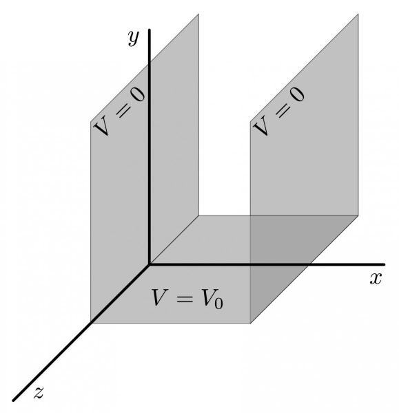
As a first example of a boundary-value problem, we examine the region between two infinite conducting plates situated at $x = 0$ and $x = L$, respectively, and above a third plate situated at $y = 0$ (see Fig.10.1). The first two plates are infinite in the $y$ and $z$ directions, they are placed parallel to each other, and they are each maintained at $V = 0$. The third plate is infinite in the $z$-direction only, and it is maintained at $V = V_0$. Notice that the potential is discontinuous at $(x,y) = (0,0)$ and $(x,y) = (L,0)$; this can be achieved by inserting a thin layer of insulating material between the bottom and side plates.
We wish to find the electrostatic potential everywhere between the two side plates and above the bottom plate. This requires finding the solution to the boundary-value problem specified by Laplace's equation $\nabla^2 V = 0$ together with the boundary conditions $V(x=0, y) = 0$, $V(x=L, y) = 0$, and $V(x,y=0) = V_0$. A fourth boundary condition is implicit: the potential should vanish at $y = \infty$, so that $V(x, y=\infty) = 0$. Because all plates are infinite in the $z$-direction, nothing changes physically as we move in that direction, and the system is therefore symmetric with respect to translations in the $z$-direction. This implies that the potential will be a function of $x$ and $y$, but will be independent of $z$.
We begin with the factorized solutions of Eqs.(10.18) and (10.19), which we write in the hybrid form
\begin{equation} V_{\alpha,\beta}(x,y,z) = \left\{ \begin{array}{l} \cos(\alpha x) \\ \sin(\alpha x) \end{array} \right\} \left\{ \begin{array}{l} e^{i\beta y} \\ e^{-i\beta y} \end{array} \right\} \left\{ \begin{array}{l} e^{\sqrt{\alpha^2+\beta^2}\, z} \\ e^{-\sqrt{\alpha^2+\beta^2}\, z} \end{array} \right\}. \tag{10.20} \end{equation}
The translational symmetry demands that we kill the $z$-dependence of these solutions, and we can achieve this by setting $\beta^2 = -\alpha^2$, so that $\beta = \pm i \alpha$. Making the substitution yields
\begin{equation} V_\alpha(x,y) = \left\{ \begin{array}{l} \cos(\alpha x) \\ \sin(\alpha x) \end{array} \right\} \left\{ \begin{array}{l} e^{\alpha y} \\ e^{-\alpha y} \end{array} \right\}, \tag{10.21} \end{equation}
where we indicate that the solutions depend on $x$ and $y$ only, and that $\alpha$ is the only remaining free parameter.
At this stage we may begin to incorporate the boundary conditions. We know that $V$ must vanish at $y = \infty$, and this implies that the solution cannot include a factor $e^{\alpha y}$, which grows to infinity. The potential must also vanish at $x = 0$, and this rules out the presence of a factor $\cos(\alpha x)$. With two boundary conditions accounted for, we find that the basis of factorized solutions must be limited to
\begin{equation} V_\alpha(x,y) = \sin(\alpha x)\, e^{-\alpha y}. \tag{10.22} \end{equation}
The parameter $\alpha$ is still arbitrary, but it is now required to be positive, to ensure that $V \to 0$ when $y \to \infty$.
The third boundary condition is that $V = 0$ at $x = L$. To achieve this we must require that $\sin(\alpha x) = 0$ at $x = L$, so that $\alpha L$ must be a multiple of $\pi$. We express this as
\begin{equation} \alpha = \frac{n\pi}{L}, \qquad n = 1, 2, 3, \cdots, \tag{10.23} \end{equation}
in terms of a positive integer $n$. (Negative integers are excluded, because $\alpha$ must be positive.) The basis of solutions is further restricted to
\begin{equation} V_n(x,y) = \sin\Bigl( \frac{n\pi x}{L} \Bigr)\, e^{-n\pi y/L},\tag{10.24} \end{equation}
and members of the basis can now be labelled with the integer $n$.
The final solution to our boundary-value problem will be a superposition of these basis solutions. We can express it as
\begin{equation} V(x,y) = \sum_{n=1}^\infty b_n \sin\Bigl( \frac{n\pi x}{L} \Bigr)\, e^{-n\pi y/L}, \tag{10.25} \end{equation}
where $b_n$ are constant coefficients. This expansion is reminiscent of a sine Fourier series --- refer back to Sec.7.9 --- but the basis functions are functions of both $x$ and $y$.
We have a fourth boundary condition to impose, that $V = V_0$ when $y = 0$. This last condition will determine the coefficients $b_n$ and finally produce a unique solution to the boundary-value problem. Setting $y=0$ in Eq.(10.25) gives
\begin{equation} V_0 = \sum_{n=1}^\infty b_n \sin\Bigl( \frac{n\pi x}{L} \Bigr), \tag{10.26} \end{equation}
and this is precisely a sine Fourier series for the constant function $V_0$. The coefficients are obtained with the help of Eq.(7.47),
\begin{equation} b_n = \frac{2}{L} \int_0^L V_0 \sin\Bigl( \frac{n\pi x}{L} \Bigr)\, dx, \tag{10.27} \end{equation}
and a short calculation yields $b_n = 2V_0(1-\cos n\pi)/(n \pi)$. For $n$ even we have that $\cos n\pi = 1$ and $b_n = 0$, while for $n$ odd we have that $\cos n\pi = -1$ and $b_n = 4V_0/(n\pi)$.
Exercise 10.1: Verify these results for the expansion coefficients $b_n$.
The final solution to the boundary-value problem is
\begin{equation} V(x,y) = \frac{4V_0}{\pi} \sum_{n=1, 3, 5, \cdots}^\infty \frac{1}{n} \sin\Bigl( \frac{n\pi x}{L} \Bigr)\, e^{-n\pi y/L}. \tag{10.28} \end{equation}
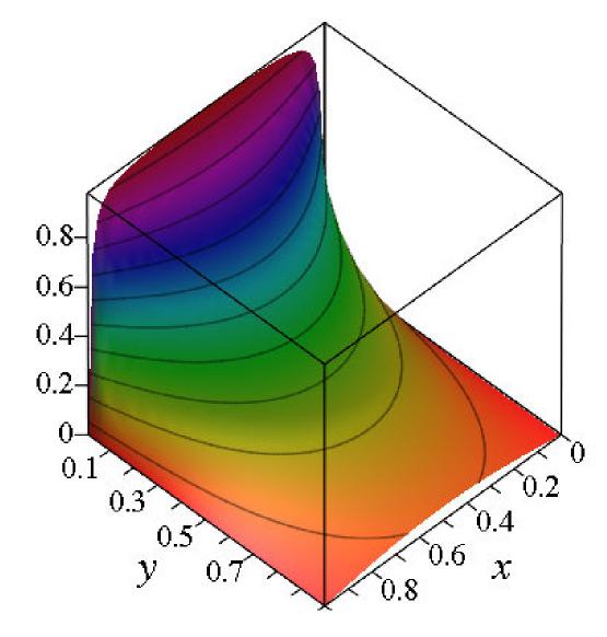
Notice that this expression is completely determined: there are no free parameters, and we do have a unique solution. It is typical for problems of this type to have a final solution expressed as an infinite series. You will recall from Chapters 7 and 8 that truncated versions of such series often make excellent approximations to the actual function. This is the case here also, as suggested by the fact that the coefficients decrease as $1/n$ with increasing $n$. The coefficients would decrease even faster if the potential didn't present discontinuities at $(x,y) = (0,0)$ and $(x,y) = (L,0)$. A three-dimensional plot of $V(x,y)$ is shown in Fig.10.2.
Remarkably, and this is not typical of such problems, the series of Eq.(10.28) can be summed explicitly. We shall not go through the details here, but merely state that the solution to our boundary-value problem can also be written as
\begin{equation} V(x,y) = \frac{2V_0}{\pi} \text{arctan} \biggl[ \frac{ \sin(\pi x/L) }{ \sinh( \pi y/L ) } \biggr]. \tag{10.29} \end{equation}
Exercise 10.2: Verify that Eq.(10.29) satisfies $\nabla^2 V = 0$ and the boundary conditions specified at the beginning of the section. Because we have in Eq.(10.29) a correct solution to the boundary-value problem, and because that solution is unique, Eq.(10.29) is necessarily equivalent to Eq.(10.28). You may find the identity \[ \frac{d}{du} \text{arctan}(u) = \frac{1}{1 + u^2} \] useful to work through this problem.
10.4 Rectangular Box
Our second example is concerned with a rectangular box of width $a$ and height $b$ constructed from conducting plates (see Fig.10.3). Each side of the box is maintained at $V=0$, except for the top side, which is maintained at $V=V_0$. We wish to find $V$ everywhere within the box.

Once again we begin with the factorized solutions of Eq.(10.19). In this case the conducting plates are all finite, and there is no translational symmetry; the potential will therefore depend on all three coordinates. And once again the factorized solutions will gradually be refined by imposing the boundary conditions; because the box has six sides, there are six conditions to impose on the potential. The first one is that $V = 0$ at $x=0$, and it implies that $\cos(\alpha x)$ must be eliminated from the factorized solutions. The second one is that $V = 0$ at $y=0$, and this eliminates $\cos(\beta y)$ from the factorized solutions. At this stage we are left with
\begin{equation} V_{\alpha,\beta}(x,y,z) = \sin(\alpha x) \sin(\beta y) \left\{ \begin{array}{l} e^{\sqrt{\alpha^2+\beta^2}\, z} \\ e^{-\sqrt{\alpha^2+\beta^2}\, z} \end{array} \right\} , \tag{10.30} \end{equation}
where $\alpha$ and $\beta$ are arbitrary parameters.
The third boundary condition is that $V = 0$ at $x = a$, and it implies that $\alpha = n\pi/a$ with $n = 1, 2, 3, \cdots$. The fourth condition is that $V = 0$ at $y = a$, and this yields $\beta = m\pi/a$ with $m = 1, 2, 3, \cdots$. The parameters $\alpha$ and $\beta$ are now determined in terms of the positive integers $n$ and $m$, and the factorized solutions become
\begin{equation} V_{n,m}(x,y,z) = \sin\Bigl( \frac{n\pi x}{a} \Bigr) \sin\Bigl( \frac{m\pi y}{a} \Bigr) \left\{ \begin{array}{l} e^{\sqrt{n^2+m^2}\, \pi z/a} \\ e^{-\sqrt{n^2+m^2}\, \pi z/a} \end{array} \right\} . \tag{10.31} \end{equation}
Notice that we have excluded negative values of $n$ and $m$. The reason is that these do not produce new factorized solutions, but merely reproduce the solutions already provided by the positive values of $n$ and $m$. To see this, consider, for example, a factorized solution corresponding to $n=-3$. This is proportional to $\sin(-3\pi x/a) = -\sin(3\pi x/a)$, which differs by a minus sign from the factorized solution corresponding to $n=+3$. Because the factorized solutions are defined up to an arbitrary numerical factor, this minus sign is of no significance, and the solution for $n=-3$ is the same as the solution for $n=3$.
The final solution to our boundary-value problem will be a superposition of the factorized solutions displayed in Eq.(10.31). We write this as
\begin{align} V(x,y,z) &= \sum_{n=1}^\infty \sum_{m=1}^\infty \biggl[ A_{nm} \sin\Bigl( \frac{n\pi x}{a} \Bigr) \sin\Bigl( \frac{m\pi y}{a} \Bigr) e^{\sqrt{n^2+m^2}\, \pi z/a} \nonumber \\ & \quad \mbox{} + B_{nm} \sin\Bigl( \frac{n\pi x}{a} \Bigr) \sin\Bigl( \frac{m\pi y}{a} \Bigr) e^{-\sqrt{n^2+m^2}\, \pi z/a} \biggr], \tag{10.32} \end{align}
where $A_{nm}$ and $B_{nm}$ are arbitrary expansion coefficients. To determine these we must proceed with the remaining boundary conditions.
The fifth boundary condition is that $V=0$ at $z=0$. Evaluating the potential of Eq.(10.32) at $z=0$ yields
\begin{equation} 0 = \sum_{n=1}^\infty \sum_{m=1}^\infty \bigl( A_{nm} + B_{nm} \bigr) \sin\Bigl( \frac{n\pi x}{a} \Bigr) \sin\Bigl( \frac{m\pi y}{a} \Bigr), \tag{10.33} \end{equation}
and we find that the expansion coefficients must be related by $B_{nm} = -A_{nm}$. Incorporating this in Eq.(10.32) gives
\begin{equation} V(x,y,z) = \sum_{n=1}^\infty \sum_{m=1}^\infty A_{nm} \sin\Bigl( \frac{n\pi x}{a} \Bigr) \sin\Bigl( \frac{m\pi y}{a} \Bigr) \Bigl( e^{\sqrt{n^2+m^2}\, \pi z/a} - e^{-\sqrt{n^2+m^2}\, \pi z/a} \Bigr), \tag{10.34} \end{equation}
or
\begin{equation} V(x,y,z) = \sum_{n=1}^\infty \sum_{m=1}^\infty 2 A_{nm} \sin\Bigl( \frac{n\pi x}{a} \Bigr) \sin\Bigl( \frac{m\pi y}{a} \Bigr) \sinh\Bigl( \sqrt{n^2+m^2}\, \frac{\pi z}{a} \Bigr) \tag{10.35} \end{equation}
if we make use of the definition $\sinh(u) := \frac{1}{2}(e^u - e^{-u})$.
The solution is now determined up to the expansion coefficients $A_{nm}$. We are getting close to the final solution, and all that remains to be done is to determine the infinite number of quantities contained in $A_{nm}$. For this we must impose the sixth and final boundary condition, that $V = V_0$ at $z = b$. Evaluating the potential of Eq.(10.35) at $z = b$ yields
\begin{equation} V_0 = \sum_{n=1}^\infty \sum_{m=1}^\infty 2 A_{nm} \sin\Bigl( \frac{n\pi x}{a} \Bigr) \sin\Bigl( \frac{m\pi y}{a} \Bigr) \sinh\Bigl( \sqrt{n^2+m^2}\, \frac{\pi b}{a} \Bigr),\tag{10.36} \end{equation}
or
\begin{equation} V_0 = \sum_{n=1}^\infty \sum_{m=1}^\infty \hat{A}_{nm} \sin\Bigl( \frac{n\pi x}{a} \Bigr) \sin\Bigl( \frac{m\pi y}{a} \Bigr) \tag{10.37} \end{equation}
if we introduce the notation
\begin{equation} \hat{A}_{nm} := 2 A_{nm} \sinh\Bigl(\sqrt{n^2+m^2}\, \frac{\pi b}{a} \Bigr). \tag{10.38} \end{equation}
Equation (10.37) is a double sine Fourier series for the constant function $V_0$. It is not difficult to show that the coefficients $\hat{A}_{nm}$ are determined by
\begin{equation} \hat{A}_{nm} = \frac{4}{a^2} \int_0^a \int_0^a V_0\, \sin\Bigl( \frac{n\pi x}{a} \Bigr) \sin\Bigl( \frac{m\pi y}{a} \Bigr)\, dx dy, \tag{10.39} \end{equation}
and a quick calculation reveals that $\hat{A}_{nm} = 16 V_0/(nm \pi^2)$ when $n$ and $m$ are both odd; otherwise the coefficients vanish.
Exercise 10.3: Prove that the expansion coefficients of the double sine Fourier series of Eq.(10.37) are given by Eq.(10.39). Actually, it is just as easy to establish the relationship for any function of $x$ and $y$; compare with Eq.(7.47). Then show that the expansion coefficients for the constant function $V_0$ are given explicitly by $\hat{A}_{nm} = 16 V_0/(nm \pi^2)$ when $n$ and $m$ are both odd.
Our result for $\hat{A}_{nm}$ implies that
\begin{equation} 2 A_{nm} = \frac{16 V_0}{\pi^2} \frac{1}{nm} \frac{1}{ \sinh\bigl( \sqrt{n^2+m^2}\, \pi b/a \bigr)}, \tag{10.40} \end{equation}
and substitution into Eq.(10.35) yields
\begin{equation} V(x,y,z) = \frac{16 V_0}{\pi^2} \sum_{n=1,3,\cdots}^\infty \sum_{m=1,3,\cdots}^\infty \frac{1}{nm} \sin\Bigl( \frac{n\pi x}{a} \Bigr) \sin\Bigl( \frac{m\pi y}{a} \Bigr) \frac{ \sinh\bigl( \sqrt{n^2+m^2}\, \pi z/a \bigr) }{ \sinh\bigl( \sqrt{n^2+m^2}\, \pi b/a \bigr) } \tag{10.41} \end{equation}
for the final solution to our boundary-value problem. We see that the solution is fully determined, and expressed as a double sum over odd integers. In this case this is the best we can do; there is no simpler expression for the solution, analogous to Eq.(10.29) in the case of the parallel plates. Representations of the potential are shown in Fig.10.4.

10.5 Cylindrical Coordinates
While Cartesian coordinates are a good choice when Laplace's equation is supplied with boundary conditions on planar surfaces, other coordinates can be better suited to other geometries. In this section we suppose that the boundary surfaces are cylinders, and consider solving Laplace's equation using the cylindrical coordinates $(s,\phi,z)$. The Laplacian operator was expressed in these coordinates back in Eq.(1.75), and we have
\begin{equation} 0 = \nabla^2 V = \frac{1}{s} \frac{\partial}{\partial s} \biggl( s \frac{\partial V}{\partial s} \biggr) + \frac{1}{s^2} \frac{\partial^2 V}{\partial \phi^2} + \frac{\partial^2 V}{\partial z^2} \tag{10.42} \end{equation}
for Laplace's equation.
The factorized solutions are of the form
\begin{equation} V = S(s) \Phi(\phi) Z(z), \tag{10.43} \end{equation}
the product of functions of $s$, $\phi$, and $z$. Substitution within Laplace's equation gives
\begin{equation} 0 = \frac{1}{sS} \frac{d}{ds} \biggl( s \frac{dS}{ds} \biggr) + \frac{1}{s^2 \Phi} \frac{d^2 \Phi}{d\phi^2} + \frac{1}{Z} \frac{d^2 Z}{dz^2}, \tag{10.44} \end{equation}
or
\begin{equation} -\frac{1}{\Phi} \frac{d^2 \Phi}{d\phi^2} = \frac{s}{S} \frac{d}{ds} \biggl( s \frac{dS}{ds} \biggr) + \frac{s^2}{Z} \frac{d^2 Z}{dz^2}. \tag{10.45} \end{equation}
This equation states that the function of $\phi$ on the left-hand side is equal to the function of $s$ and $z$ on the right-hand side. This gives rise to the same kind of contradiction that we encountered before in Sec.10.2, and to escape it we must declare that these functions are in fact constant.
Writing the constant as $m^2$, we have that
\begin{equation} \frac{1}{\Phi} \frac{d^2 \Phi}{d\phi^2} = -m^2, \tag{10.46} \end{equation}
which has
\begin{equation} \Phi(\phi) = e^{\pm im\phi} \tag{10.47} \end{equation}
or
\begin{equation} \Phi(\phi) = \left\{ \begin{array}{l} \cos(m\phi) \\ \sin(m\phi) \end{array} \right. \tag{10.48} \end{equation}
for solutions. Now, $\phi$ is the angle from the $x$-axis, and as such it is limited to the interval $0 \leq \phi < 2\pi$. A trip through this interval (with $s$ and $z$ fixed) is a rotation around the $z$-axis, and arriving at $\phi = 2\pi$ is the same thing as returning to the starting position $\phi = 0$. Suppose that $V \propto \Phi(\phi)$ was equal to the value $V_0$ at the start of the trip. The potential must return to the same value $V_0$ at the end of the trip --- $V$ must have one and only one value at each point in space --- and this implies that $\Phi(\phi)$ must satisfy $\Phi(2\pi) = \Phi(0)$. With $\Phi = e^{\pm im\phi}$, this can be achieved if and only if $2m\pi$ is a multiple of $2\pi$, and this means that $m$ must be an integer, $m = 0, 1, 2, 3, \cdots$. Our conclusion is that the potential $V$ will fail to be a single-valued function unless $m$ is an integer, and that we must therefore impose this condition on the constant $m$.
With $\Phi(\phi)$ now determined in terms of $m$, Eq.(10.45) can be re-expressed as
\begin{equation} m^2 = \frac{s}{S} \frac{d}{ds} \biggl( s \frac{dS}{ds} \biggr) + \frac{s^2}{Z} \frac{d^2 Z}{dz^2}, \tag{10.49} \end{equation}
or
\begin{equation} -\frac{1}{Z} \frac{d^2 Z}{dz^2} = -\frac{m^2}{s^2} + \frac{1}{sS} \frac{d}{ds} \biggl( s \frac{dS}{ds} \biggr). \tag{10.50} \end{equation}
Here we have that the function of $z$ on the left-hand side must be equal to the function of $s$ on the right-hand side. Because $z$ and $s$ are independent variables, we have the good old contradiction arising once again, and once again we elude it by declaring that the functions are constant. We write $-k^2$ for this constant, so that
\begin{equation} \frac{1}{Z} \frac{d^2 Z}{dz^2} = k^2, \tag{10.51} \end{equation}
and get
\begin{equation} Z(z) = e^{\pm kz} \tag{10.52} \end{equation}
or
\begin{equation} Z(z) = \left\{ \begin{array}{l} \cosh(k z) \\ \sinh(k z) \end{array} \right. \tag{10.53} \end{equation}
for solutions.
Making the substitution in Eq.(10.50) gives
\begin{equation} -k^2 = -\frac{m^2}{s^2} + \frac{1}{sS} \frac{d}{ds} \biggl( s \frac{dS}{ds} \biggr), \tag{10.54} \end{equation}
or
\begin{equation} s \frac{d}{ds} \biggl( s \frac{dS}{ds} \biggr) + (k^2 s^2 - m^2) S = 0,\tag{10.55} \end{equation}
or
\begin{equation} s^2 \frac{d^2 S}{ds^2} + s \frac{dS}{ds} + (k^2 s^2 - m^2) S = 0. \tag{10.56} \end{equation}
This is a second-order differential equation for $S(s)$, and its form can be simplified by introducing the new variable $u := k s$. This yields
\begin{equation} u^2 \frac{d^2 S}{du^2} + u \frac{dS}{du} + (u^2 - m^2) S = 0, \tag{10.57} \end{equation}
and comparison with Eq.(5.26) reveals that this differential equation is none other than Bessel's equation. There are two independent solutions to this equation, and we recall from Sec.5.9 that they are denoted $J_m(u)$ and $N_m(u)$. We also recall that while $J_m(u)$ is finite at $u=0$, $N_m(u)$ is infinite there. The solutions for $S(s)$ are therefore
\begin{equation} S(s) = \left\{ \begin{array}{l} J_m(ks) \\ N_m(ks) \end{array} \right., \tag{10.58} \end{equation}
and we have obtained the factorized solutions to Laplace's equation in cylindrical coordinates.
Collecting results, we have that the factorized solutions are given by
\begin{equation} V_{m,k}(s,\phi,z) = \left\{ \begin{array}{l} J_m(ks) \\ N_m(ks) \end{array} \right\} \left\{ \begin{array}{l} e^{im\phi} \\ e^{-im\phi} \end{array} \right\} \left\{ \begin{array}{l} e^{kz} \\ e^{-kz} \end{array} \right\}, \tag{10.59} \end{equation}
where $m = 0, 1, 2, 3, \cdots$ and $k$ is an arbitrary parameter. They can also be expressed as
\begin{equation} V_{m,k}(s,\phi,z) = \left\{ \begin{array}{l} J_m(ks) \\ N_m(ks) \end{array} \right\} \left\{ \begin{array}{l} \cos(m\phi) \\ \sin(m\phi) \end{array} \right\} \left\{ \begin{array}{l} \cosh(kz) \\ \sinh(kz) \end{array} \right\}, \tag{10.60} \end{equation}
or in a hybrid form that would blend together exponential, trigonometric, and hyperbolic functions. The factorized solutions of Eqs.(10.59) and (10.60) form the building blocks from which we can obtain the solution to any boundary-value problem in cylindrical coordinates.
10.6 Cylindrical Pipe
As an example of a boundary-value problem in cylindrical coordinates, we examine a semi-infinite, cylindrical pipe of radius $R$ (see Fig.10.5). The wall of the pipe at $s = R$ is maintained at $V = 0$, and the base of the pipe at $z = 0$ is maintained at $V = V_0$. We wish to solve Laplace's equation $\nabla^2 V = 0$ to find the potential everywhere within the pipe.

We begin with the factorized solutions of Eq.(10.59), which we will gradually refine by imposing the boundary conditions. We note first that the boundary conditions do not involve the angle $\phi$. This reveals the existence of a rotational symmetry: nothing changes physically as we rotate around the $z$-axis, and it follows that the potential cannot depend on $\phi$. This implies that $m$ must be set equal to zero in the factorized solutions. A second observation is that the potential is expected to go to zero as $z \to \infty$, and this implies that we must eliminate $e^{kz}$ from the factorized solutions. A third observation is that $V$ should not become infinite on the pipe's axis ($s=0$), and this allows us to eliminate $N_m(ks)$ from the factorized solutions. At this stage we have obtained that the solution to the boundary-value problem must be built from
\begin{equation} V_k(s,z) = J_0(ks)\, e^{-kz}, \tag{10.61} \end{equation}
where $k$ is an arbitrary parameter.
The potential is required to go to zero at $s = R$. This can be achieved by demanding that $kR$ be a zero of the Bessel function, so that $k = \alpha_{0p}/R$, where, in the notation introduced in Sec.5.3, $\alpha_{0p}$ is the $p^{\rm th}$ zero of the zeroth Bessel function. The factorized solutions become
\begin{equation} V_p(s,z) = J_0(\alpha_{0p} s/R)\, e^{-\alpha_{0p} z/R}, \tag{10.62} \end{equation}
and they are now labelled with the integer $p = 1, 2, 3, \cdots$. The solution to the boundary-value problem will be a superposition of these,
\begin{equation} V(s,z) = \sum_{p=1}^\infty c_p J_0(\alpha_{0p} s/R)\, e^{-\alpha_{0p} z/R}, \tag{10.63} \end{equation}
with $c_p$ denoting the expansion coefficients.
To determine $c_p$ we must impose the final boundary condition, that $V = V_0$ at $z = 0$. This leads to
\begin{equation} V_0 = \sum_{p=1}^\infty c_p J_0(\alpha_{0p} s/R), \tag{10.64} \end{equation}
a Bessel series for the constant function $V_0$. Techniques to invert Bessel series were described back in Sec.8.4, and Eq.(8.24) informs us that the coefficients are given by
\begin{equation} c_p = \frac{2}{\bigl[ J_1(\alpha_{0p}) \bigr]^2} \int_0^1 V_0 J_0(\alpha_{0p} u)\, u\, du, \tag{10.65} \end{equation}
where $u := s/R$. We rewrite this as
\begin{equation} c_p = \frac{2V_0}{\bigl[ \alpha_{0p} J_1(\alpha_{0p}) \bigr]^2} \int_0^{\alpha_{0p}} v J_0(v)\, dv \tag{10.66} \end{equation}
by introducing the new integration variable $v := \alpha_{0p} u$. We rely on the recursion relation of Eq.(5.20d) with $n=1$ to write $v J_0 = (v J_1)'$ and evaluate the integral. We arrive at
\begin{equation} c_p = \frac{2V_0}{\alpha_{0p} J_1(\alpha_{0p})} \tag{10.67} \end{equation}
for the expansion coefficients.
Inserting Eq.(10.67) within Eq.(10.63) gives
\begin{equation} V(s,z) = 2 V_0 \sum_{p=1}^\infty \frac{1}{\alpha_{0p} J_1(\alpha_{0p})} J_0(\alpha_{0p} s/R)\, e^{-\alpha_{0p} z/R} \tag{10.68} \end{equation}
for the unique solution to the boundary-value problem, expressed as an infinite sum of products of Bessel and exponential functions. The potential can be evaluated at any $s$ and $z$ using a truncated version of this sum, and the result of this computation is displayed in Fig.10.6.

10.7 Spherical Coordinates
Spherical boundaries call for spherical coordinates, and in this section we take on the task of solving Laplace's equation in these coordinates. The Laplacian operator expressed in terms of $(r,\theta,\phi)$ was obtained back in Eq.(1.86), and we have
\begin{equation} 0 = \nabla^2 V = \frac{1}{r^2} \frac{\partial}{\partial r} \biggl( r^2 \frac{\partial V}{\partial r} \biggr) + \frac{1}{r^2\sin\theta} \frac{\partial}{\partial \theta} \biggl( \sin\theta \frac{\partial V}{\partial \theta} \biggr) + \frac{1}{r^2\sin^2\theta} \frac{\partial^2 V}{\partial \phi^2} \tag{10.69} \end{equation}
for Laplace's equation.
As usual we begin with a factorized solution of the form
\begin{equation} V(r,\theta,\phi) = R(r) Y(\theta,\phi), \tag{10.70} \end{equation}
which we shall insert within Laplace's equation. We could factorize $Y(\theta,\phi)$ further by writing it as $\Theta(\theta) \Phi(\phi)$, but this shall not be necessary. The notation might trigger some expectation that $Y$ will have something to do with spherical harmonics.
Substitution into Laplace's equation yields
\begin{equation} 0 = \frac{1}{R} \frac{d}{dr} \biggl( r^2 \frac{dR}{dr} \biggr) + \frac{1}{Y} \biggl[ \frac{1}{\sin\theta} \frac{\partial}{\partial \theta} \biggl( \sin\theta \frac{\partial Y}{\partial \theta} \biggr) + \frac{1}{\sin^2\theta} \frac{\partial^2 Y}{\partial \phi^2} \biggr], \tag{10.71} \end{equation}
and this equation informs us that a function of $r$ only must be equal to a function of $\theta$ and $\phi$. As usual we conclude that each function must be a constant, which we denote $\mu$. We therefore obtain the ordinary differential equation
\begin{equation} \frac{d}{dr} \biggl( r^2 \frac{dR}{dr} \biggr) = \mu R \tag{10.72} \end{equation}
for the radial function, and the partial differential equation
\begin{equation} \frac{1}{\sin\theta} \frac{\partial}{\partial \theta} \biggl( \sin\theta \frac{\partial Y}{\partial \theta} \biggr) + \frac{1}{\sin^2\theta} \frac{\partial^2 Y}{\partial \phi^2} = -\mu Y \tag{10.73} \end{equation}
for the angular function. This equation may be compared with Eq.(4.44), the differential equation satisfied by the spherical harmonics. They are identical in form, except that here, $\mu$ is not necessarily equal to $\ell(\ell+1)$, with $\ell$ a nonnegative integer.
It can be shown that for a generic value of $\mu$, the solutions to Eq.(10.73) become infinite at $\theta = \pi$ when they are required to be finite at $\theta = 0$. We made a similar observation before, back in Sec.3.9, in the context of Legendre functions. There we noted that the generalized Legendre equation,
\begin{equation} (1-u^2) f'' - 2u f' + \lambda(\lambda+1) f = 0, \tag{10.74} \end{equation}
has solutions that must blow up at $u=-1$ even when they are finite at $u = 1$, unless $\lambda$ is a nonnegative integer. A generalization to the associated Legendre equation,
\begin{equation} (1-u^2) f'' - 2u f' + \biggl[ \lambda(\lambda+1) - \frac{m^2}{1-u^2} \biggr] f = 0, \tag{10.75} \end{equation}
makes the situation even worse. With $u = \cos\theta$, we are speaking of functions that become infinite at $\theta = \pi$, just like the $Y$ of Eq.(10.73).
The singular solutions to Eq.(10.73) are simply not acceptable; our potential should be nicely behaved everywhere in space, and it should certainly not go to infinity on the negative $z$-axis. This compels us to set $\mu$ equal to $\ell(\ell+1)$, because in this case Eq.(10.73) becomes <\p> \begin{equation} \frac{1}{\sin\theta} \frac{\partial}{\partial \theta} \biggl( \sin\theta \frac{\partial Y}{\partial \theta} \biggr) + \frac{1}{\sin^2\theta} \frac{\partial^2 V}{\partial \phi^2} = -\ell(\ell+1) Y, \tag{10.76} \end{equation}
which is precisely the differential equation for the spherical harmonics. The solutions are $Y^m_\ell(\theta,\phi)$, with $\ell = 0, 1, 2, 3, \cdots$ and $m = -\ell,-\ell+1,\cdots,\ell-1,\ell$, and these are all nicely behaved functions that don't go infinite anywhere. With this restriction on $\mu$, Eq.(10.72) becomes
\begin{equation} r^2 \frac{d^2 R}{dr^2} + 2r \frac{dR}{dr} = \ell(\ell+1) R, \tag{10.77} \end{equation}
and it is easy to show that this differential equation possesses the independent solutions $R = r^\ell$ and $R = r^{-(\ell+1)}$.
Exercise 10.4: Find the two solutions to Eq.(10.77). The form of the differential equation suggests the use of $r^\alpha$ as a trial solution, where $\alpha$ is a constant.
The factorized solutions to Laplace's equation in spherical coordinates are therefore
\begin{equation} V^m_\ell(r,\theta,\phi) = \left\{ \begin{array}{l} r^\ell \\ r^{-(\ell+1)} \end{array} \right\} Y^m_\ell(\theta,\phi), \tag{10.78} \end{equation}
and they are labelled by the integers $\ell$ and $m$ that enter the specification of the spherical harmonics. A solution to a boundary-value problem formulated in spherical coordinates will be a superposition of these basis solutions. We write it as
\begin{equation} V(r,\theta,\phi) = \sum_{\ell=0}^\infty \sum_{m=-\ell}^\ell \Bigl[ A^m_\ell\, r^\ell + B^m_\ell\, r^{-(\ell+1)} \Bigr] Y^m_\ell(\theta,\phi), \tag{10.79} \end{equation}
and the expansion coefficients $A^m_\ell$ and $B^m_\ell$ will be determined by the boundary conditions specific to each problem.
10.7 Hemispheres

As a first example of a boundary-value problem formulated in spherical coordinates, we examine a system consisting of two conducting hemispheres of radius $R$ joined together at the equator (see Fig.10.7). The upper hemisphere is maintained at $V = V_0$, while the lower hemisphere is maintained at $V = -V_0$. There is a thin layer of insulating material between the two hemispheres, to allow for the discontinuity of the potential at the equator. We wish to find the potential everywhere inside the sphere.
Because the boundary conditions don't refer to $\phi$, and because a rotation around the $z$-axis doesn't change the situation physically, the potential will be independent of $\phi$. This implies that only terms with $m = 0$ will survive in the expansion of Eq.(10.79). And because the potential should not blow up at the centre of the sphere, we must also kill all $r^{-(\ell+1)}$ terms by setting $B^m_\ell = 0$. Recalling that $Y^0_\ell \propto P_\ell(\cos\theta)$, we are looking for a solution of the form
\begin{equation} V(r,\theta) = \sum_{\ell=0}^\infty c_\ell (r/R)^\ell P_\ell(\cos\theta), \tag{10.80} \end{equation}
where $c_\ell \propto A^0_\ell$ are the expansion coefficients, and where the factor of $R^{-\ell}$ was inserted for convenience.
To determine the expansion coefficients we must impose the boundary conditions, $V(R,\theta) = V_0$ when $0 \leq \theta < \pi/2$ and $V(R,\theta) = -V_0$ when $\pi/2 \leq \theta < \pi$. Introducing the new variable $u := \cos\theta$, we have that the potential on the hemispheres is equal to the function $f(u)$ defined by $f(u) = -V_0$ when $-1 < u \leq 0$ and $f(u) = V_0$ when $0 < u \leq 1$. The boundary conditions and Eq.(10.80) imply that
\begin{equation} f(u) = \sum_{\ell=0}^\infty c_\ell P_\ell(u), \tag{10.81} \end{equation}
which is recognized as a Legendre series for the function $f(u)$. Techniques to invert Legendre series were described back in Sec.8.2, and Eq.(8.10) informs us that the expansion coefficients are given by
\begin{equation} c_\ell = \frac{1}{2} (2\ell+1) \int_{-1}^1 f(u) P_\ell(u)\, du. \tag{10.82} \end{equation}
A straightforward calculation, which follows the same steps as those presented in an example in Sec.~\ref{sec8:legendre}, reveals that $c_\ell = 0$ when $\ell$ is even, and that
\begin{equation} c_\ell = V_0 \bigl[ P_{\ell-1}(0) -P_{\ell+1}(0) \bigr] \tag{10.83} \end{equation}
when $\ell$ is odd.
Exercise 10.5: Show that $c_0 = 0$. Then use the recursion relation of Eq.(3.21b) to prove that for $\ell \geq 1$, $c_\ell = V_0[P_{\ell-1}(0) -P_{\ell+1}(0)]$. From the properties of the Legendre polynomials at $u=0$, conclude that $c_\ell = 0$ when $\ell$ is even. Verify that $c_1 = \frac{3}{2} V_0$, $c_3 = -\frac{7}{8} V_0$, $c_5 = \frac{11}{16} V_0$, and $c_7 = -\frac{75}{128} V_0$.
The potential inside the hemispheres is therefore given by
\begin{equation} V(r,\theta) = V_0 \sum_{\ell=1, 3, 5, \cdots}^\infty \bigl[ P_{\ell-1}(0) -P_{\ell+1}(0) \bigr] (r/R)^\ell P_\ell(\cos\theta). \tag{10.84} \end{equation}
A three-dimensional plot of the potential is shown in Fig.10.8.

10.8 Angle-Dependent Boundary Conditions
As a second example of boundary-value problem, we wish to solve Laplace's equation $\nabla^2 V = 0$ inside a sphere of radius $R$, on which the potential is equal to $V(R,\theta,\phi) = V_0 \sin^2\theta \cos^2\phi$. Because the potential is not constant on the surface of the sphere, we are clearly not dealing with a conducting surface.
The solution to this problem will be of the form of Eq.(10.79), with $B^m_\ell$ set to zero to avoid a singularity at $r = 0$. We need to determine $A^m_\ell$, and for this we must identify the spherical harmonics that will actually participate in the solution. The main clue is provided by the boundary condition, once it is decomposed in spherical harmonics. This exercise was actually carried out back in Sec.8.3, where we found that the boundary potential can be written as
\begin{equation} V(R,\theta,\phi) = V_0 \biggl[ \frac{1}{3} - \frac{1}{6} (3\cos^2\theta - 1) + \frac{1}{2} \sin^2\theta \cos(2\phi) \biggr]. \tag{10.85} \end{equation}
While this expression doesn't seem to involve spherical harmonics, in fact they are there in disguise. Comparison with the listing provided in Sec.4.6 --- refer back to Eq.(4.36) --- reveals that $\frac{1}{3}$ is proportional to $Y^0_0$, $\frac{1}{6} (3\cos^2\theta - 1)$ is proportional to $Y^0_2$, and that $\frac{1}{2} \sin^2\theta \cos(2\phi)$ is proportional to $Y^2_2 + Y^{-2}_2$. The important point is that up to numerical factors, the first term in the decomposition of $\sin^2\theta \cos^2\phi$ is a spherical harmonic with $\ell = 0$, while the remaining terms are spherical harmonics with $\ell = 2$.
How do we turn this information into a solution to Laplace's equation? The answer is: easily! We inspect Eq.(10.79) with $B^m_\ell = 0$ and deduce that the only values of $\ell$ and $m$ implicated in this sum will be those that are forced on us by the boundary condition, namely $(\ell,m) = (0,0)$, $(2,0)$, and $(2,\pm 2)$. We also deduce that the relevant spherical harmonics will present themselves in the combinations identified previously; in particular, $Y^2_2$ and $Y^{-2}_2$ will come together to form $\frac{1}{2} \sin^2\theta \cos(2\phi)$. Furthermore, we observe from Eq.(10.79) that a spherical harmonic of degree $\ell$ always comes with a factor of $r^\ell$ in front. We can always write this factor as $(r/R)^\ell$ instead, at the cost of multiplying the unknown coefficients $A^m_\ell$ by a compensating factor of $R^\ell$. We now have all the ingredients: the relevant spherical harmonics, and the appropriate factors of $(r/R)^\ell$ in front of them.
To obtain the final solution to the boundary-value problem we simply take each term in Eq.(10.85) and multiply it by the appropriate factor of $(r/R)^\ell$. This gives
\begin{equation} V(r,\theta,\phi) = V_0 \biggl[ \frac{1}{3} - \frac{1}{6} (r/R)^2 (3\cos^2\theta - 1) + \frac{1}{2} (r/R)^2 \sin^2\theta \cos(2\phi) \Biggr], \tag{10.86} \end{equation}
which we claim is the unique solution to Laplace's equation that satisfies the stated boundary conditions.
Exercise 10.6: In case you are skeptical that the method described above leads to the correct solution, verify that the potential of Eq.(10.86) satisfies $\nabla^2 V = 0$ and becomes $V_0 \sin^2\theta \cos^2\phi$ when $r = R$. Do this even if you are not skeptical: this is a good exercise for the soul.
This problem could have been solved more formally by inverting the spherical-harmonic series along the lines described in Sec.8.3. Because this method requires, in principle, the calculation of an infinite number of expansion coefficients, one for each value of $\ell$ and $m$, it can be a bit laborious to implement in practice. It really pays off to use the boundary conditions to identify the relevant spherical harmonics first, as we have done here. Once this is done, the solution to the boundary-value problem presents itself simply by incorporating the appropriate factors of $r^\ell$ or $r^{-(\ell+1)}$. The method can be adapted to many different situations.
10.9 Conductor In a Uniform Electric Field
For a final example we consider a conducting sphere of radius $R$ that is immersed within a uniform electric field $\boldsymbol{E} = E \boldsymbol{\hat{z}}$, where $E = \text{constant}$. Before the immersion the field was truly constant, but the arrival of the conductor distorts the electric field, because of the induced charge distribution on the surface; the final field is not quite uniform. We wish to calculate the electric potential $V$, under the assumption that the conductor is maintained at $V=0$ during the immersion. Recall that the potential is related to the electric field by $\boldsymbol{E} = -\boldsymbol{\nabla} V$.
The condition $V=0$ at $r=R$ provides one of the boundary conditions, but we must also account for the fact that at large distances from the conductor, the electric field will approach the uniform configuration $\boldsymbol{E} = E \boldsymbol{\hat{z}}$ that was present before the immersion. (The impact of the conductor on the electric field can be expected to behave as $q/(4\pi \epsilon_0 r^2)$ at large distances, with $q$ denoting the total surface charge.) To represent this constant field at large distances we need a potential that behaves as $V \sim -E z$, or
\begin{equation} V \sim - E\, r \cos\theta, \qquad r \to \infty. \tag{10.87} \end{equation}
This asymptotic condition will play the role of a second boundary condition. Notice that the potential does not go to zero at infinity; instead it must be proportional to $z = r\cos\theta$, so as to give rise to a constant electric field at infinity.
The situation is symmetric under rotations around the $z$-axis, and to reflect this the potential must be independent of $\phi$. The general expansion of Eq.(10.79) therefore reduces to
\begin{equation} V(r,\theta) = \sum_{\ell=0}^\infty \Bigl[ A_\ell\, r^\ell + B_\ell\, r^{-(\ell+1)} \Bigr] P_\ell(\cos\theta), \tag{10.88} \end{equation}
an expansion in Legendre polynomials. The asymptotic condition tells us that we must include the $r P_1 = r\cos\theta$ term in the sum, and exclude all $r^\ell P_\ell$ terms with $\ell \geq 2$. The boundary condition at $r=R$ further tells us that we must also include the $r^{-2} P_1 = r^{-2} \cos\theta$ term, and exclude all remaining $r^{-(\ell+1)} P_\ell$ terms. The asymptotic and boundary conditions do not instruct us to exclude the $\ell = 0$ terms, and we find that the final solution must be the form
\begin{equation} V = A_0 + B_0/r + \bigl( A_1 r + B_1/r^2 \bigr) \cos\theta. \tag{10.89} \end{equation}
The constant $A_1$ can be determined from the asymptotic condition, and we find that $A_1 = -E$. The constant $B_1$ is then determined from the requirement that $V = 0$ at $r = R$; this yields $B_1 = E R^3$. The same condition implies that $B_0 = -A_0 R$, and we now have
\begin{equation} V = A_0 (1 - R/r) - E (r - R^3/r^2) \cos\theta \tag{10.90} \end{equation}
Notice that $V$ depends on an unknown constant $A_0$ that is not determined by the boundary and asymptotic conditions. To give it an interpretation, let us write $A_0 := -q/(4\pi \epsilon_0 R)$, and therefore express $A_0$ in terms of another constant $q$ with the dimension of charge. The final form of the solution shall then be
\begin{equation} V(r,\theta) = \frac{1}{4\pi \epsilon_0} \frac{q}{r} \biggl( 1 - \frac{r}{R} \biggr) - E \biggl( 1 - \frac{R^3}{r^3} \biggr) r \cos\theta. \tag{10.91} \end{equation}
In this form we can recognize the meaning of the constant $q$, which represents the total charge of the system, distributed on the surface of the spherical conductor. The $q/(4\pi \epsilon_0 r)$ term in the potential comes with a correction proportional to $r/R$, and this represents an irrelevant constant. The second set of terms is more interesting. We recognize the $-E\, r\cos\theta$ contribution to the potential, which gives rise to the constant field at large distances, but we also see a correction proportional to $R^3/r^3$, which comes from the distribution of surface charge on the conductor.
This problem is interesting because of the physics that it contains, but it is also interesting from a purely mathematical point of view. The reason is that it seems to provide a violation of the uniqueness theorem: the potential involves the unknown total charge $q$, and therefore the solution to the boundary-value problem is not unique. Do we have a genuine violation? The answer is no, because we are trespassing beyond the limits of the theorem. The uniqueness theorem requires a strict specification of boundary conditions. In this problem, however, we substituted a strict boundary condition with the asymptotic condition of Eq.(10.87). Because this condition does not specify a value for $V$ at a specific place, but merely tells us how the potential grows with $z = r\cos\theta$ at large distances, it does not give us enough information to pin down the potential uniquely. Additional information, like the value of the total charge $q$, is therefore required for a unique solution.
10.10 Practice Problems
-
(Boas Chapter 12, Section 2, Problem 3) Consider the problem of the parallel plates, as in Sec.10.3, but assume now that the bottom plate is maintained at $V = V_0 \cos x$. Find the potential in the region between the side plates and above the bottom plate.
-
(Boas Chapter 12, Section 2, Problem 7) Solve Laplace's equation for a potential $V(x,y)$ that satisfies the boundary conditions $V(x=0, y) = 0$, $V(x=\pi,y) = 0$, $V(x, y=0) = \cos x$, and $V(x, y=1) = 0$. Find the potential in the region described by $0 < x < \pi$ and $0 < y < 1$.
-
(Boas Chapter 12, Section 2, Problem 11) Solve Laplace's equation for a potential $V(x,y)$ that satisfies the boundary conditions $V(x=0, y) = V_0$, $V(x=1,y) = 0$, $V(x, y=0) = V_0$, and $V(x, y=1) = 0$. Find the potential in the region described by $0 < x < 1$ and $0 < y < 1$.
-
(Boas Chapter 12, Section 5, Problem 1a) Calculate numerically the first five coefficients $c_p$ in the cylindrical pipe problem, as given by Eq.~(\ref{eq10:Vcyl_pipe_coeffs}). Evaluate the potential at $s = \frac{1}{2} R$ and $z = R$.
-
(Boas Chapter 12, Section 5, Problem 2b) Consider a semi-infinite cylindrical pipe of radius $R$. The wall of the pipe is maintained at $V = 0$, and its base is maintained at $V = V_0 (s/R) \sin\phi$. Find the potential inside the pipe.
-
(Boas Chapter 12, Section 7, Problem 1) Solve Laplace's equation inside a sphere of radius $R$ when the potential on the surface is given by $V(r=R,\theta) = 35\cos^4\theta$.
-
(Boas Chapter 12, Section 7, Problem 2) Solve Laplace's equation inside a sphere of radius $R$ when the potential on the surface is given by $V(r=R,\theta) = \cos\theta - \cos^3\theta$.
-
(Boas Chapter 12, Section 7, Problem 10) Solve Laplace's equation outside a sphere of radius $R$ when the potential on the surface is given by $V(r=R,\theta,\phi) = 3\sin\theta\cos\theta\sin\phi$.
-
(Boas Chapter 12, Section 7, Problem 10) Solve Laplace's equation outside a sphere of radius $R$ when the potential on the surface is given by $V(r=R,\theta,\phi) = \sin^2\theta\cos\theta\cos(2\phi) - \cos\theta$.
10.11 Challenge Problems
-
a) Solve the two-dimensional Laplace equation $\nabla^2 V = 0$ for the function $V(x,y)$ in the domain described by $0 \leq x \leq 1$ and $0 \leq y \leq 1$. The boundary conditions are that $V = 0$ on $y = 0$, $V = 0$ on $y = 1$, $V = V_0 y(1-y^2)$ on $x = 0$, and $V = 0$ on $x = 1$. Here and below, $V_0$ is a constant. Your solution will be expressed as a Fourier series.
b) for $y=1/2$, between $x=0$ and $x=1$.
-
Solve the three-dimensional Laplace equation $\nabla^2 V = 0$ for the function $V(r,\theta,\phi)$ in the domain between a small sphere at $r = a$ and a large sphere at $r = b$. The boundary conditions are that $V = 0$ at $r=a$, and $V = V_0 \sin^2\theta \cos^2\phi$ at $r=b$. Your final answer should be expressed in terms of elementary functions (powers of $r$ and simple trigonometric functions of $\theta$ and $\phi$).
a) What are the factorized solutions for the two-dimensional Laplace equation $\nabla^2 V = 0$ expressed in polar coordinates $s$ and $\phi$?
b) Find the solution $V(s,\phi)$ to this two-dimensional Laplace equation in the domain corresponding to a half-disk of radius $1$ centred at the origin of the coordinate system. The domain's outer boundary is the half-circle described by $s = 1$, $0 \leq \phi \leq \pi$ and the straight line segment that links the points $(x=-1,y=0)$ and $(x=1,y=0)$ along the $x$-axis. The boundary conditions are that $V = V_0$ on the half-circle, and that $V = 0$on the straight segment. Your solution will be expressed as a Fourier series.
c) On the same graph, plot $V(s,\phi)$ as a function of $\phi$ (between $\phi = 0$ and $\phi = \pi$) for $s = 0.3$ and $s=0.9$.
d) On the same graph, plot $V(s,\phi)$ as a function of $s$ (between $s=0$ and $s=1$) for $\phi = 0.01$, $\phi = \pi/2$, and $\phi = 3.14$.